Data Labs

Documentation for the NERC CEH Data Labs project.

version: 0.35.7

Getting Help

I'm having trouble logging into DataLabs

In order to login to DataLabs you'll need to create an account using the sign up button from the home page. Once you've created an account, you'll need to verify your e-mail before being able to sign in.

I have signed in but can't see anything, what do I do now?

Initially, you will only be able to see projects which you own or have been given access to. If you are expecting to collaborate on an existing project, ask one of the project admins to give you permission to access the project. Otherwise, contact your DataLabs instance administrator to request a project.

Where do I get started having logged in with access to a project?

A number of tutorials will be added over time which will help with getting started within DataLabs.

I am a project owner, how do I add more people to my project?

This is done from the project page and browsing to Settings in the sidebar, from here you can type a users e-mail in the Add User field and assign them a permission.

Note that once you have added a user, what they will be able to do depends on the permission that they have been assigned, a brief summary is below;

• Admin - Has control of adding and removing users to the project as well as creating data storage.
• User - Can create and control notebooks and sites but not storage.
• Viewer - Can only view sites that are created, has no ability to create any resources.

Note that the exception to this is if a user chooses to share their notebook with the entire project, at this point every member of the project will be able to access it.

I'm a user in a project but can't create a notebook

Once you are part of a project as a user you will have the permission to create notebooks, but this may not be possible unless you have been assigned a data store to use. These are created by admins under the Storage tab. In order to be able to create a notebook, ask an admin to add you to a data store which you will be able to use.

I've never used notebooks before, where can I find out more?

A number of notebooks are available in DataLabs, links to useful introductory documentation for each of them can be found below.

• JupyterLab
• RStudio
• Zeppelin

All of them share a common theme of providing a work environment where code can be run and visualized, while also running on a platform that allows you to work collaboratively with others.

I have noticed some things which are different about working in DataLabs than locally?

There are a few key differences to know about when working within DataLabs compared to locally.

The main one concerns how packages are installed and persisted. Within DataLabs your runtime environment (i.e Python and R packages) must be stored alongside the code. Practically, this means using tools such as Conda environments or Packrat.

Is there a limit to the number of projects I can be a part of?

There is currently a limit of 50 projects that any individual user can be a part of (Admin/User/Viewer). If you are worried about hitting this limit please raise this with an administrator.

I am having problems which I can't find the answer to here, how do I get help?

We are active on Slack and happy to discuss any problems with you there where possible.

Tutorials

These pages contain tutorials for DataLabs.

The tutorials are aimed at new users, and are focused on introducing you to the key functionality within DataLabs. They take the form of clear, step-by-step instructions, with an emphasis on how to achieve a relatively simple goal.

My First Notebook

This tutorial is recommended for all first-time users of DataLabs.

In this tutorial you will create a JupyterLab notebook within DataLabs. This will give you an initial view of some of the concepts within DataLabs, which will help you in your general use.

1. Sign up to DataLabs
2. Log in to DataLabs
3. Access a project
4. Open your project
5. Create project storage
6. Create a JupyterLab
7. Start a Jupyter notebook
8. Collaborative JupyterLab
9. Conclusion

1. Sign up to DataLabs

In this section you will obtain a DataLabs account.

If you already have a DataLabs account, you can skip this section.

In your browser, navigate to https://datalab.datalabs.ceh.ac.uk (or whatever your local instance of DataLabs is).

Click the Sign Up button. Depending on your local instance of DataLabs, follow the instructions to create an account.

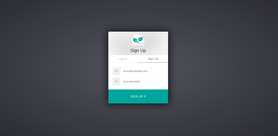
For CEH DataLabs, you will be taken to a page on auth0.com:

Navigate to the Sign Up tab, and enter an email address (this will be your username) and a password. The email address must be for an account you can access, as you will be sent a verification email.

You will then be taken to a page asking you to verify your email address.

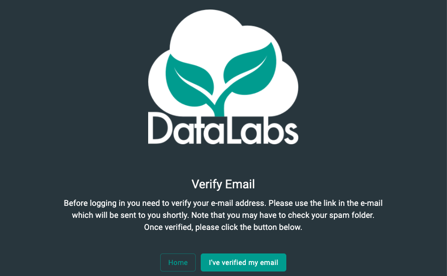
In your email client, you should receive an email with a verification link or button, which you should click. You will be taken to a page informing you that your email was verified.

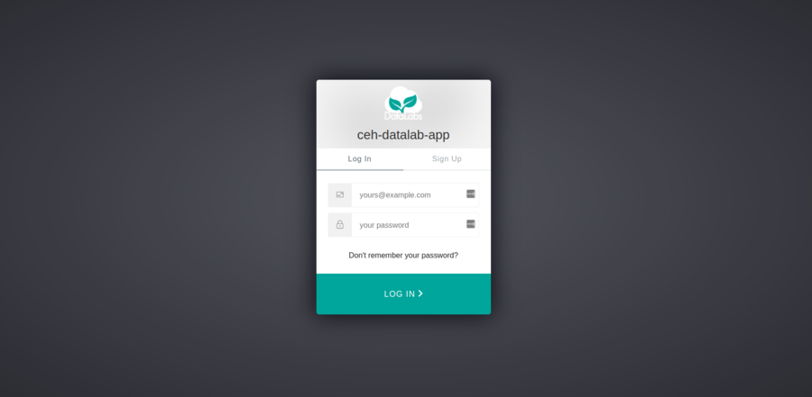
Back on the DataLabs page, you can now click the "I've verified my email button". This will take you to a login page.

2. Log in to DataLabs

In this section you will log in to DataLabs.

If you have already logged in to DataLabs, you can skip this section.

Starting point: you should already have a DataLabs account. If you have just finished the preceding section, you will already be on the auth0 log in page. Otherwise, navigate to https://datalab.datalabs.ceh.ac.uk (or whatever your local instance of DataLabs is), and click the Log In button.

You will then be taken to a page asking you to enter your username (email address) and password.

Enter your email address and password, and click the LOG IN button. You will then arrive at the DataLabs Projects page.

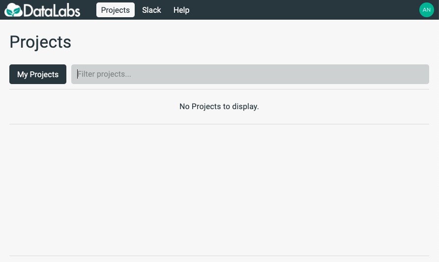
3. Access a project

In this section you will ensure you have access to a project. A project is a container for your storage and notebooks, allowing for sharing and collaboration with other users.

Starting point: you should be logged in to DataLabs, at the projects home page.

If you already have a project, it will be visible on your projects home page:

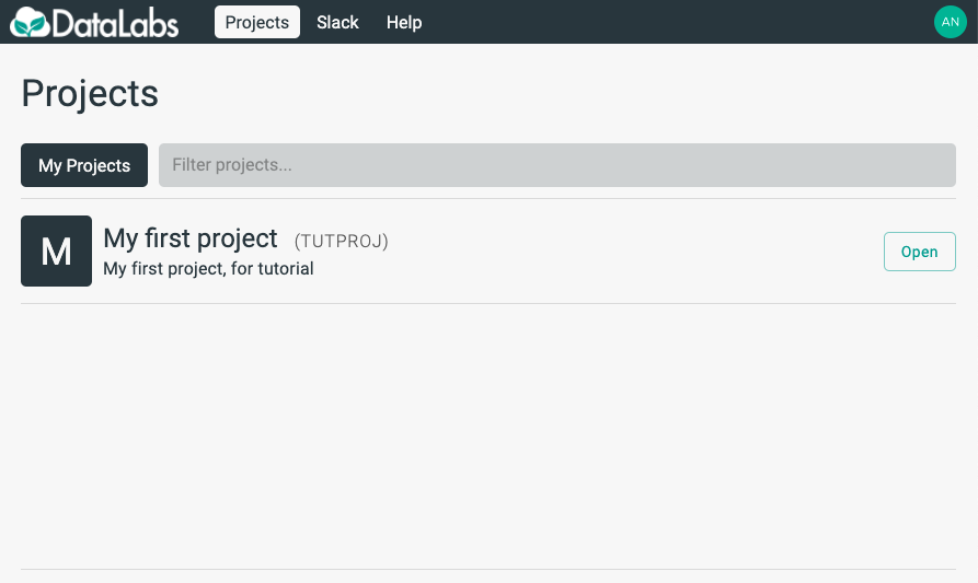
If you do not already have a project, you should ask an administrator to create a project for you. Once that has happened, you can proceed with the tutorial.

4. Open your project

In this section you will open your project and check you have the right permissions to continue with the tutorial.

Starting point: you should be logged in to DataLabs, at the projects home page, with a project visible.

Click on the Open button. You will be taken to that project page.

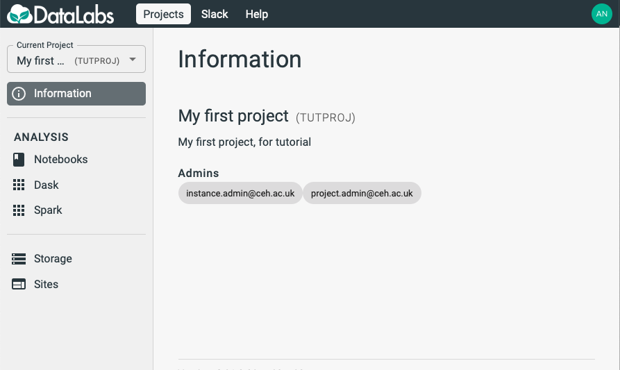
Verify that your email address is listed as a project admin (like project.admin@ceh.ac.uk is in the above screenshot). If you are listed as a user or a viewer, you will not have permission to create storage for a notebook - contact one of the project admins in order to obtain the right permission.

On the left hand side of the page, you will see Notebooks and Storage. We will create and use these in the remainder of the tutorial.

5. Create project storage

In this section you will create some project storage, in order to store your notebook.

Starting point: you should be logged in to DataLabs, in a project you have admin permissions for.

On the left-hand-side, click the Storage link.

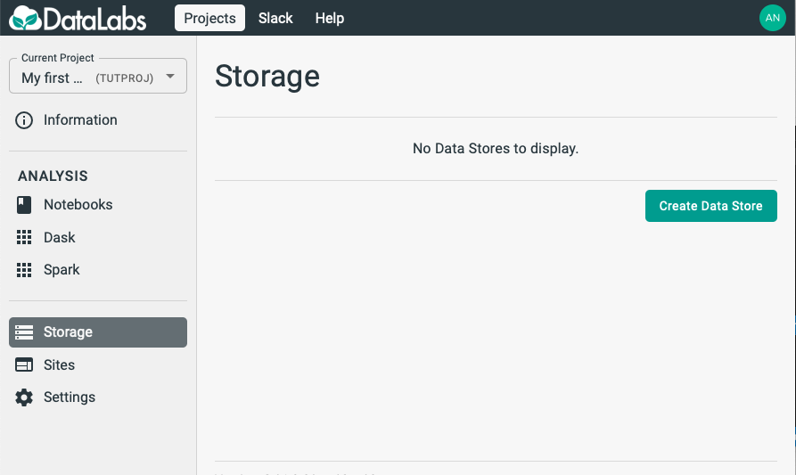
Click the Create Data Store button, and fill out a form to create storage. Then click the Create button.

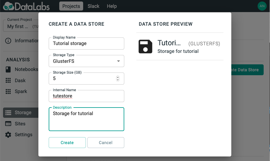
You will then be able to see the storage that you have created.

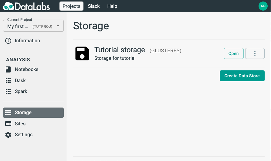
6. Create a JupyterLab

In this section you will create a JupyterLab notebook.

Starting point: you should be logged in to DataLabs, in a project you have admin permissions for, with some project storage already created.

On the left-hand-side, click the Notebooks link.

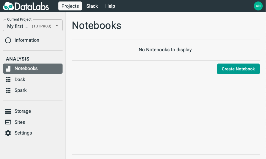
Click the Create Notebook button, and fill out a form to create a notebook. For Type, select JupyterLab. Then click the Create button.

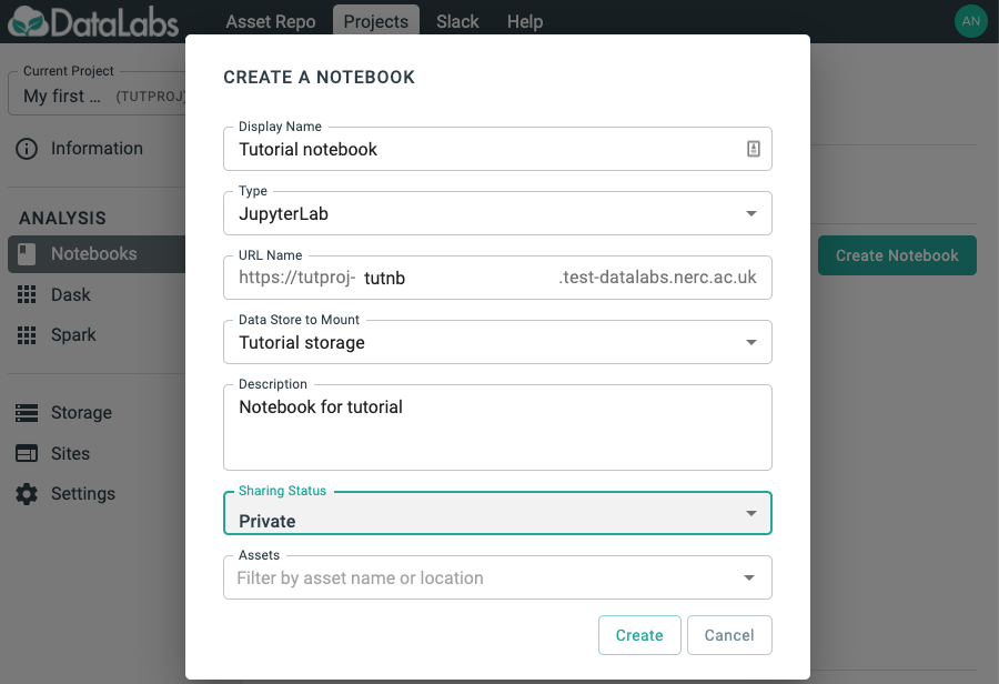
You will then be able to see the notebook that you have created.

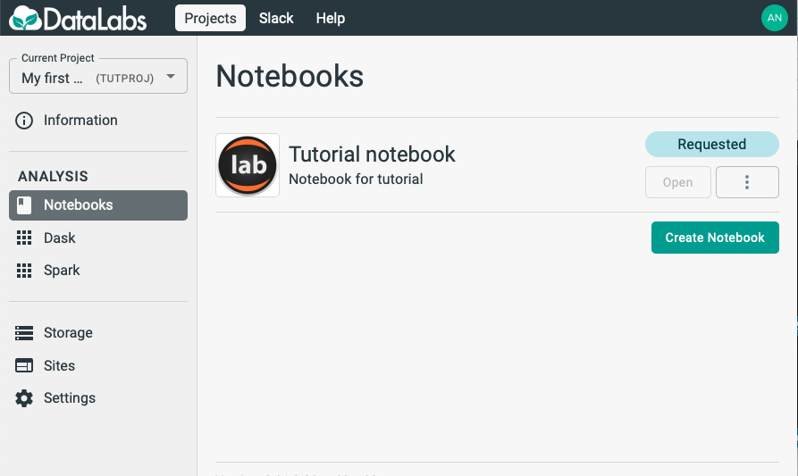
Initially the notebook will have a status of requested. You will have to wait a few minutes for the status to change to Ready before continuing with the tutorial.

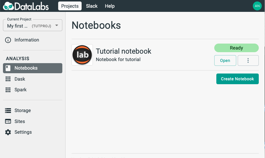
7. Start a Jupyter notebook

In this section you will start a Jupyter notebook.

Starting point: you should be logged in to DataLabs, in a project you have admin permissions for, with some project storage and a JupyterLab notebook already created.

On the right hand side, click the Open button. If your browser prevents pop-ups, you may have to enable pop-ups for this site. On a new browser tab, a JupyterLab launcher should open.

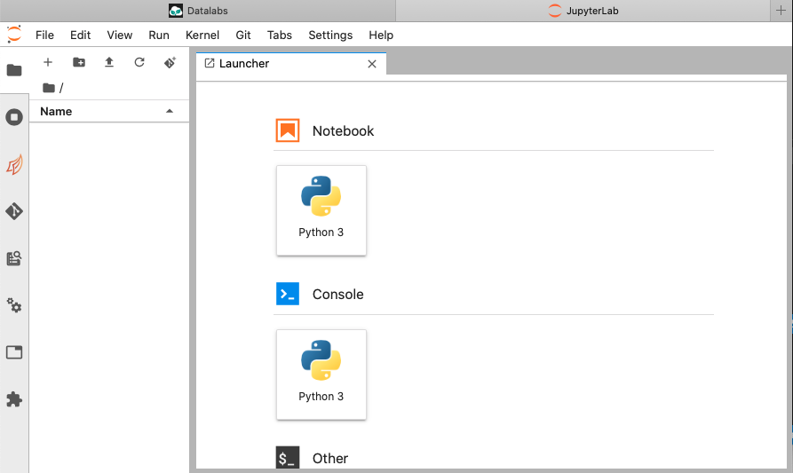
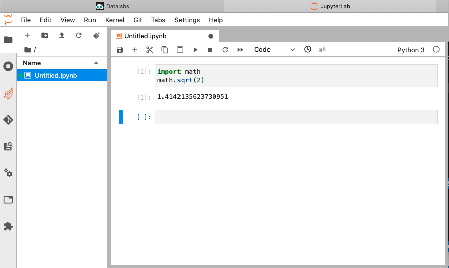
Click the Python 3 button. Within JupyterLab, a Python Jupyter notebook is created.

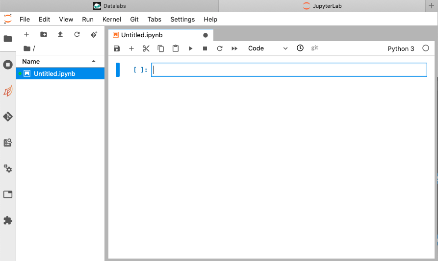
You can enter a Python calculation in the cell, and then click the 'Play' button on the Jupyter menu bar to execute the cell contents.

Working with JupyterLab collaboratively

From JupyterLab version 3.1 onwards, notebooks are run using the --collaborative flag, meaning that multiple users can work on the same notebook at the same time, each seeing live updates as others type and execute cells.

When another user is working on the same notebook, a cursor will appear where they have selected, and will briefly show a name in a particular colour. This name is currently set to Anonymous <Name> - however, this name is chosen randomly each time the notebook is launched, so it is possible to have a different name (and colour) after relaunching the notebook, and it is also possible for multiple users to have the same name (though they may have different colours).

An example is shown below - user 1 (on the left) is currently typing, so their name "Anonymous Chaldene" appears for user 2 (on the right):

Then, user 2 (on the right) starts typing, and for user 1 (on the left), they appear as "Anonymous Arche".

8. Conclusion

Congratulations!

In this tutorial, you have:

• Created a DataLabs account.
• Logged in to DataLabs.
• Opened a project, which is a container for your storage and notebooks, allowing for sharing and collaboration with other users.
• Created some project storage.
• Created a JupyterLab notebook.
• Executed some Python in a Jupyter notebook.

Where next?

You may want to consider these next steps:

• To learn more about JupyterLab, visit https://jupyterlab.readthedocs.io/en/stable/.
• To read up on how to get started with a Python environment inside Jupyter, visit the getting started with Jupyter tutorial.

My first Visual Studio Code project

This tutorial is recommended for all users who are starting a new project in Visual Studio Code for the first time.

By the end of this tutorial you should have access to a web-baseed Visual Studio Code setup stored in DataLabs where you can edit code, customise your configuration and install extensions.

1. Create a Visual Studio Code notebook
2. Start the notebook

1. Create a new Visual Studio Code Notebook

In this section you will create a new Visual Studio Code notebook. Like JupyterLab notebooks, Visual Studio Code notebooks require a storage area to save their configuration and environment in, so make sure you are logged into a project and have created some storage.

Click on the Create Notebook button in the Notebooks section and fill out the form, making sure to choose VS Code Server as the Type.

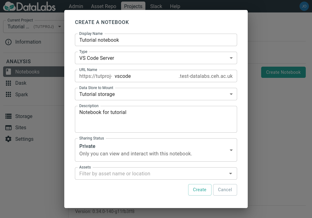
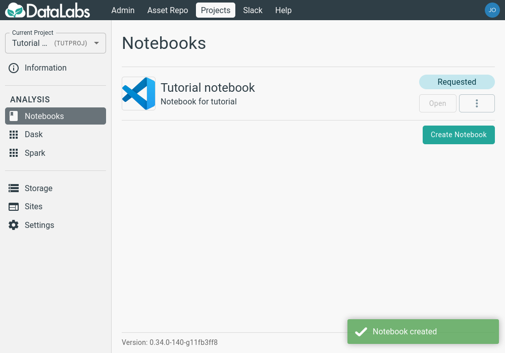
When you have entered all the required details, click the Create button, and the notebook will be requested.

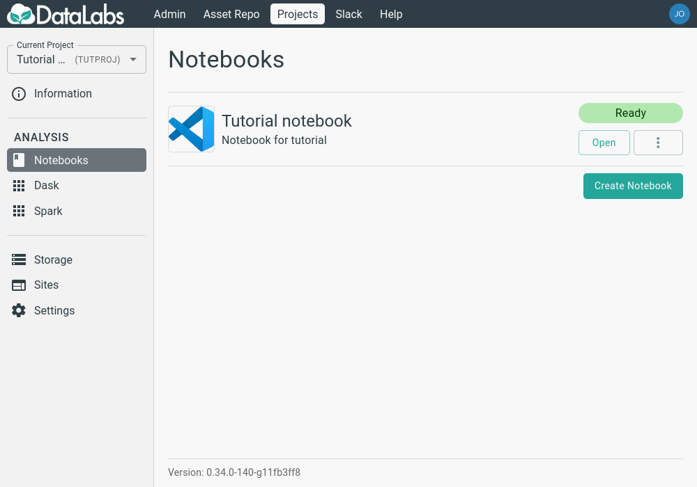
After a few minutes, the notebook will have been created and will be ready to be opened.

2. Start editing with Visual Studio Code

Once you have created a Visual Studio Code notebook, you can launch it by clicking the Open button on the right. As with JupyterLab, you may have to enable pop-ups for this site.

An instance of Visual Studio Code will open in a new browser tab.

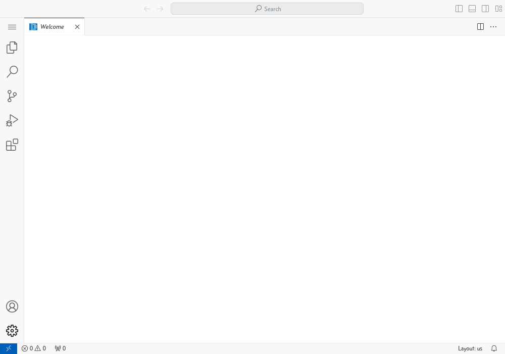
You can then create a notebook or script file, and edit it as normal in Visual Studio Code. You can install extensions and create and use Conda environments as though Visual Studio Code was running on your own computer.

My first RStudio Project

This tutorial is recommended for all users who are starting a new project in RStudio for the first time.

This tutorial will walk you through setting up a basic RStudio project which crucially uses renv, a tool designed to capture all of your packages alongside the code and which is needed within DataLabs for your project to work consistently.

1. Create a new RStudio project
2. Install some packages
3. Run some example analysis code

1. Create a new RStudio project

In this section you will create a new RStudio project. Projects are a concept within RStudio for keeping everything related to one piece of work together and integrates nicely with tools such as renv (and historically packrat).

Starting point: you should have been logged into DataLabs and created a new RStudio notebook which has been opened.

Once in RStudio, create a new project by browseing to File > New Project, and selecting New Directory. On the following form choose New Project.

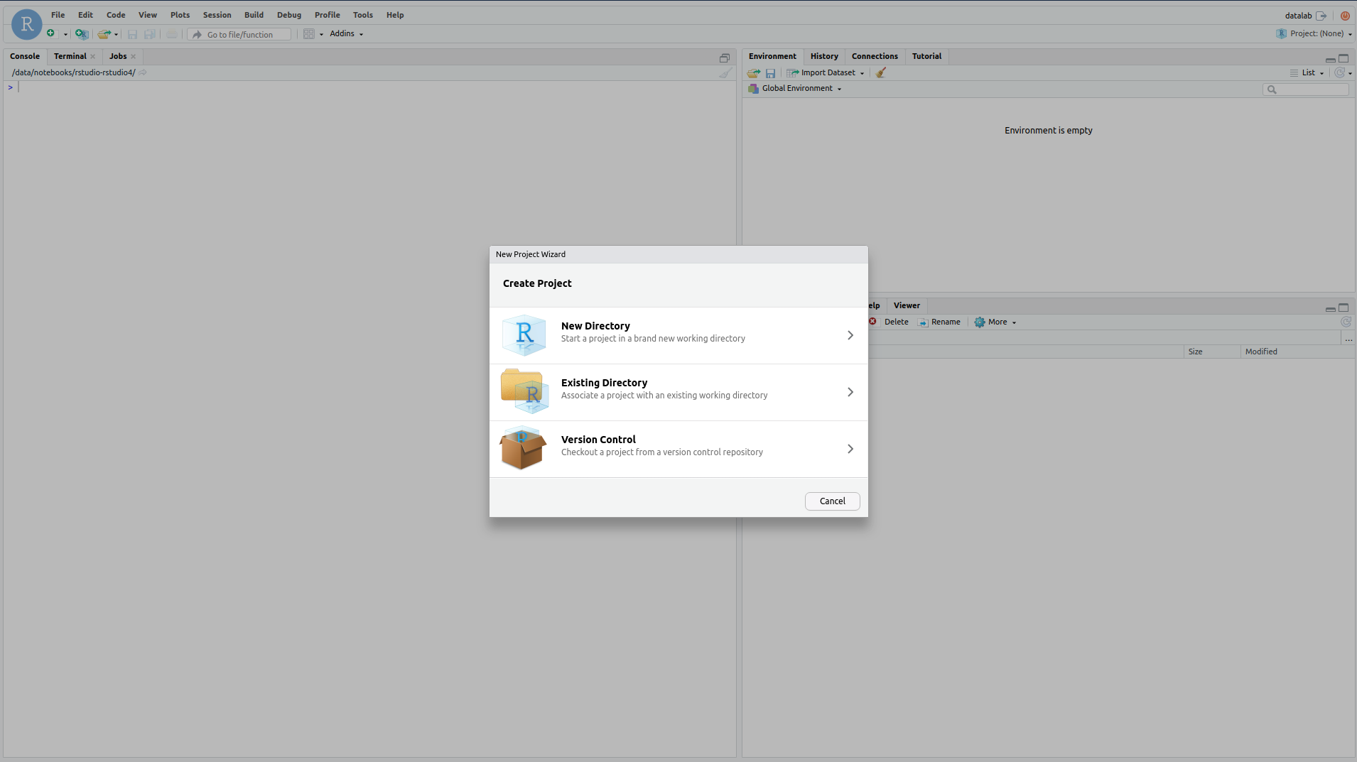
After selecting this, enter a name for the directory the project will live in and browse to select where the project directory will be saved (you may need to make a new folder). At this point select the checkbox titled Use renv with this project, at which point you can select Create Project.

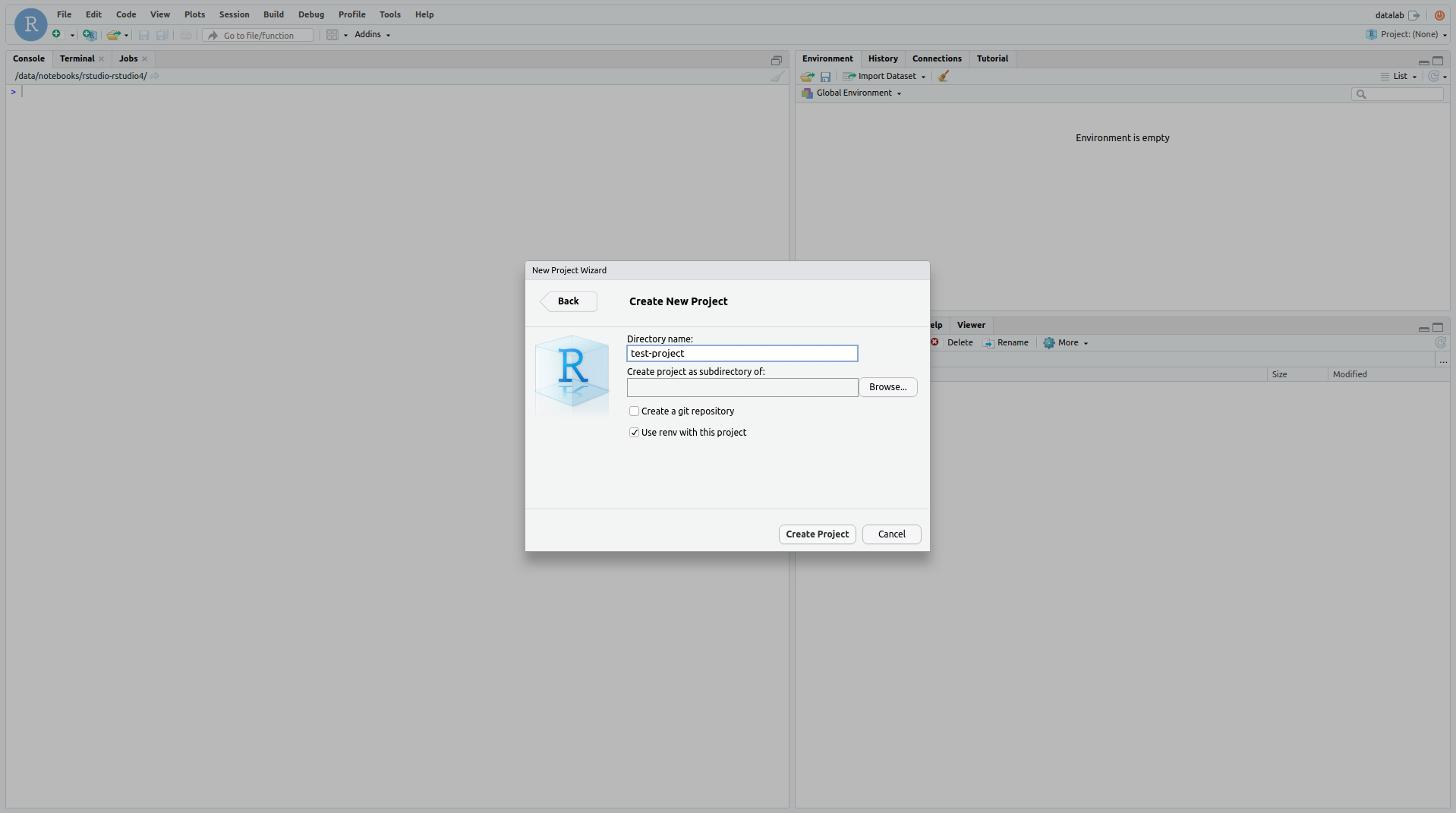
This will trigger the creation of a new RStudio project and will also trigger a refresh of your browser. Once the browser reloads you should be able to see in the top right underneath datalab that the project you are currently using is the same name you entered initially.

2. Install packages

Once you have loaded into your new project you can begin installing packages that you will need. As renv is being used in this project any new packages installed will by default be stored within the project directory without any additional configuration. Hence they can be installed as per normal e.g

install.packages("nycflights13")
install.packages("ggplot2")

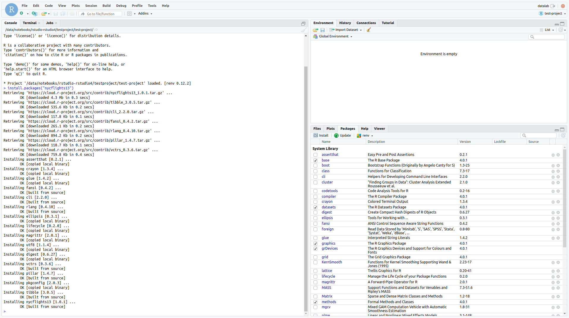
At this point you can browse to Packages on the bottom right panel which will show which packages are available in your R environment as well as their versions. This area can also be used to install new packages if you prefer. Some standard things to install can be analysis or visualization packages such as ggplot2 and data.table.

3. Example Analysis

Once you have a project set up and some basic packages installed, you can begin to create R files and carry out analysis. A good place to start is simply visualizing some data. The nycflights13 package contains some good example data relating to flights from a US airport.

Paste the code below into an R notebook and run it. It simply plots a histogram of the time difference with arrival (negative is early), it represents something looking like a normal distribution.

library(nycflights13)
library(ggplot2)
flights <- nycflights13::flights
ggplot(flights, aes(x=arr_delay), binwidth=20) + xlim(-75,150) + geom_histogram(binwidth=1)

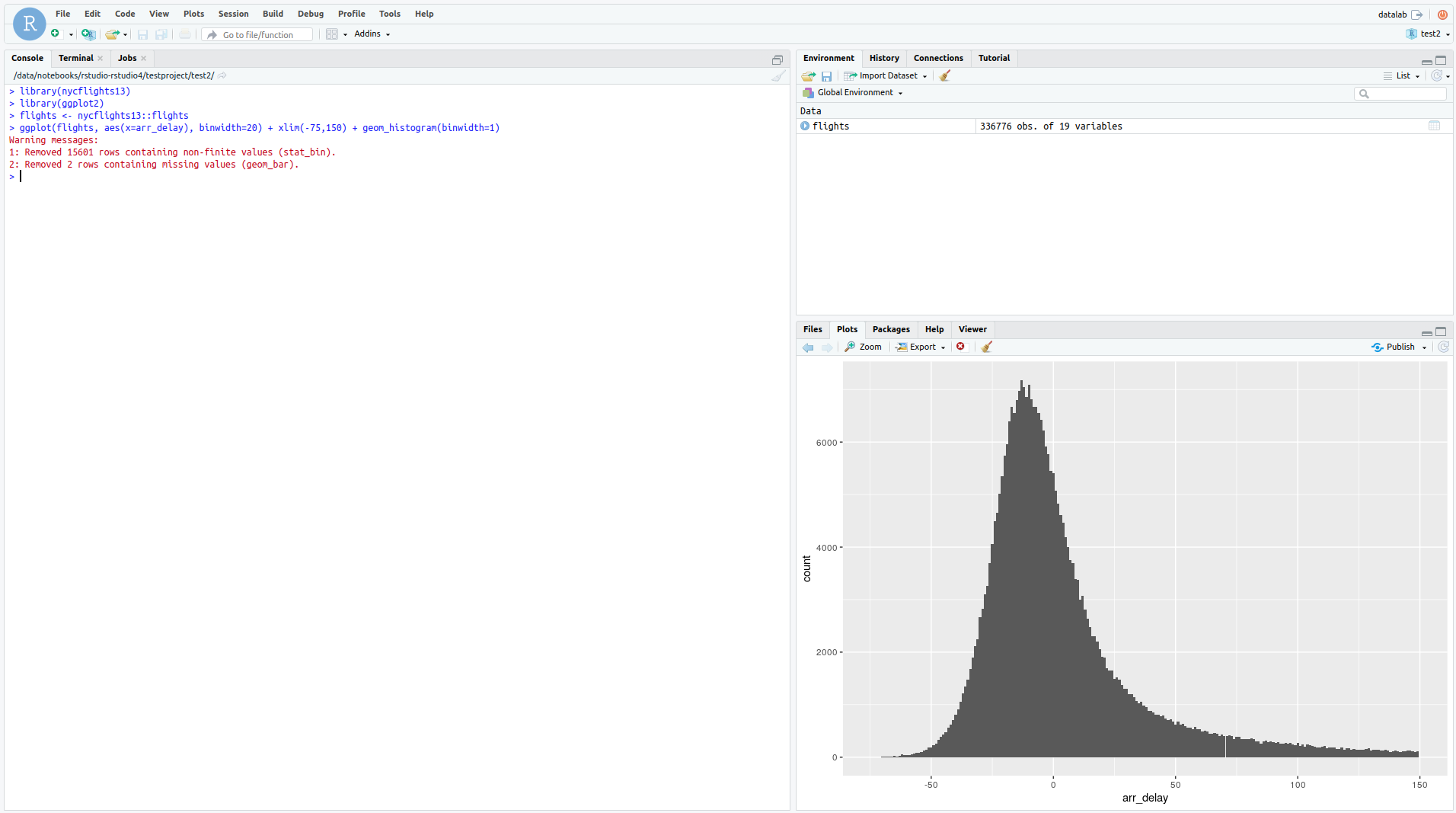
There are a number of very good tutorials which make use of the nycflights13 dataset and help you get started with using a wide arrayy of useful packages and techniques.

8. Conclusion

Congratulations!

In this tutorial, you have:

• Created a new RStudio Project
• Installed some basic packages for data analysis
• Run some basic code to generate a plot

Where next?

You may want to consider these next steps:

• To learn some more fundamentals about how RStudio works, visit https://rafalab.github.io/dsbook/getting-started.html
• To tackle some more basic data analysis, follow https://www.r-bloggers.com/2018/08/exploratory-data-analysis-in-r-introduction/

My first Jupyter Project

This tutorial is recommended for all users who are starting a new project in Jupyter for the first time and will go through some small example R and python code.

By the end of this tutorial you should have in place a conda environment, some basic R and python packages, and have run example code snippets for each.

1. Create a Conda environment
2. Install some packages
3. Run some example analysis code

1. Create Conda Environment

Open a JupyterLab notebook from DataLabs, this should send you to a landing page. From here, open up a terminal via File > New > Terminal. Within the terminal run the following command;

env-control add new-environment

This will trigger the creation of a Conda environment as well as adding Jupyter Kernels for both R & Python which are persisted on the data volume. When running this for a brand new environment this is likely to take ~10 minutes as it installs a number of dependencies.

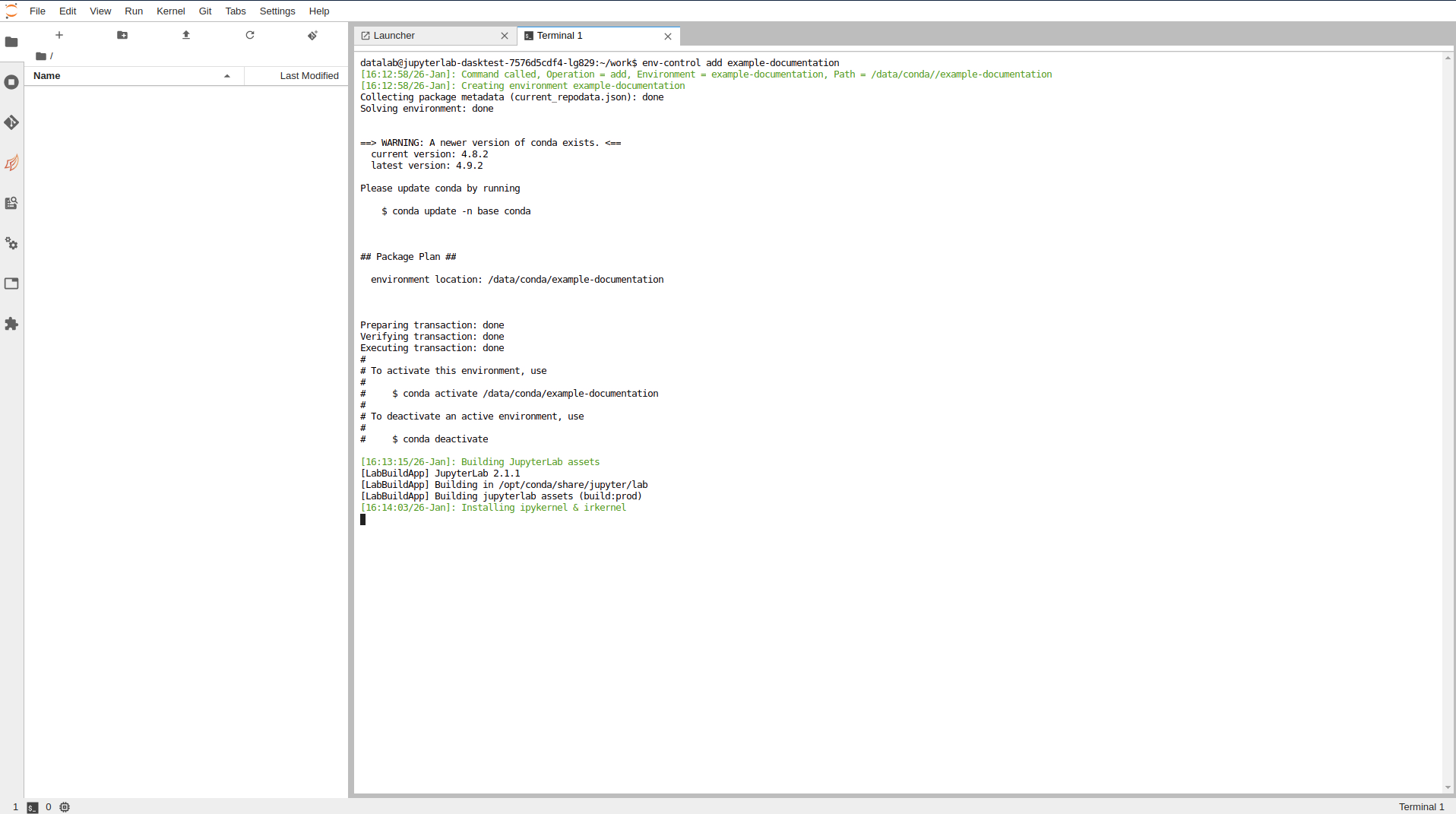
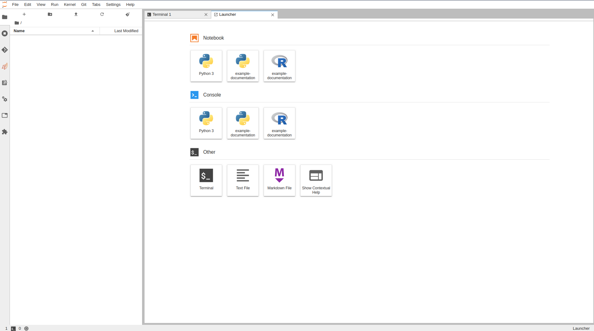
Once the command is complete, refresh the page (F5) and browse to the Launcher (File > New Launcher), from here you should see two new kernels which correspond to the newly created Conda environment, one for each of Python and R.

2. Install packages

After creating a conda environment you can then begin installing the packages that you need to use.

There are multiple methods for installing packages in a Conda environment, but this tutorial will cover the most basic case for both Python and R. In each case we will install a few example packages which we will use later in an example.

Python

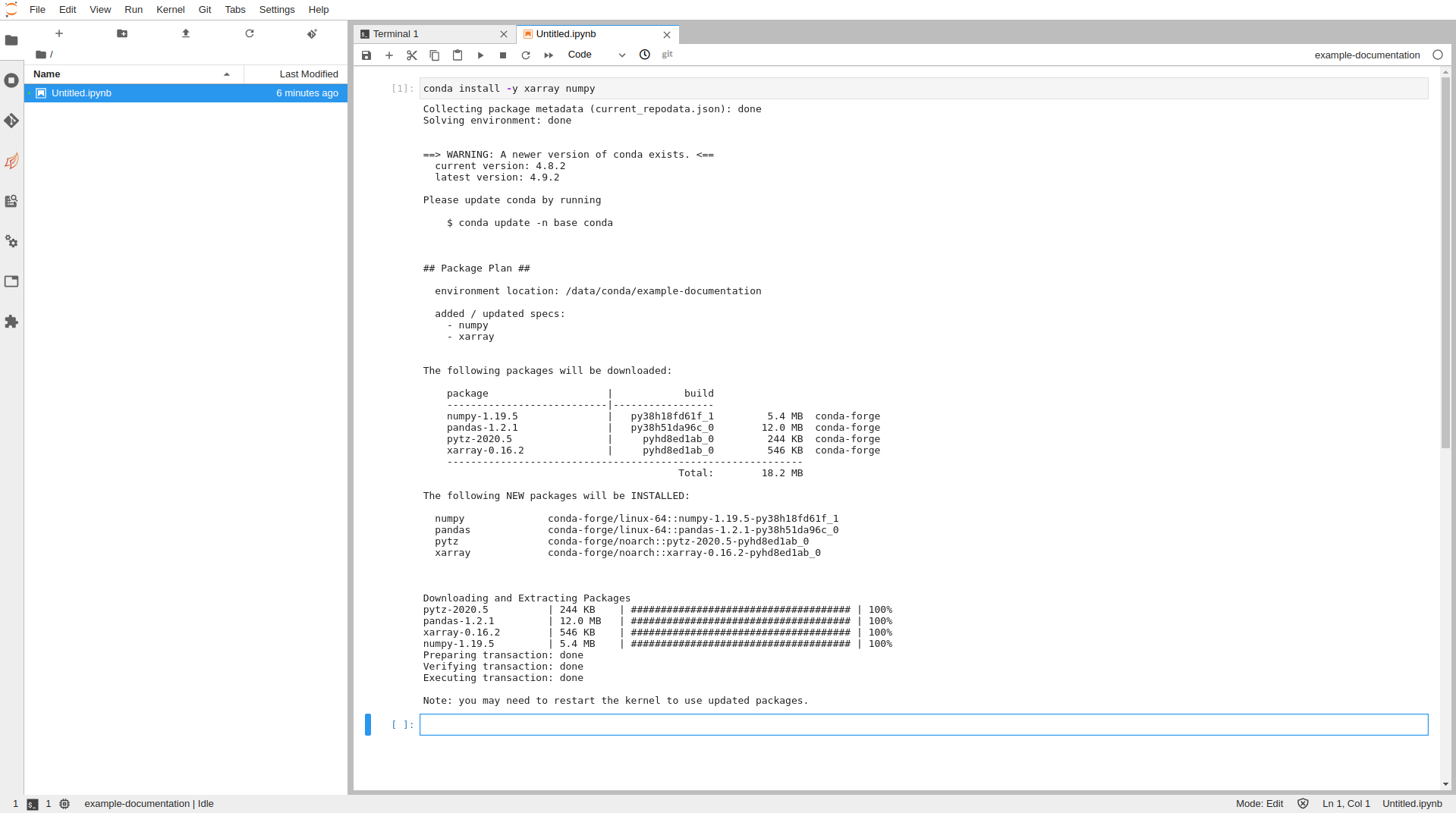
From the launcher screen for Jupyter, select the kernel associated with the environment you just created for Python. This will put you into a Python notebook where we will install a few standard packages which are common for data analysis.

conda install -y xarray numpy matplotlib pandas netcdf4

R

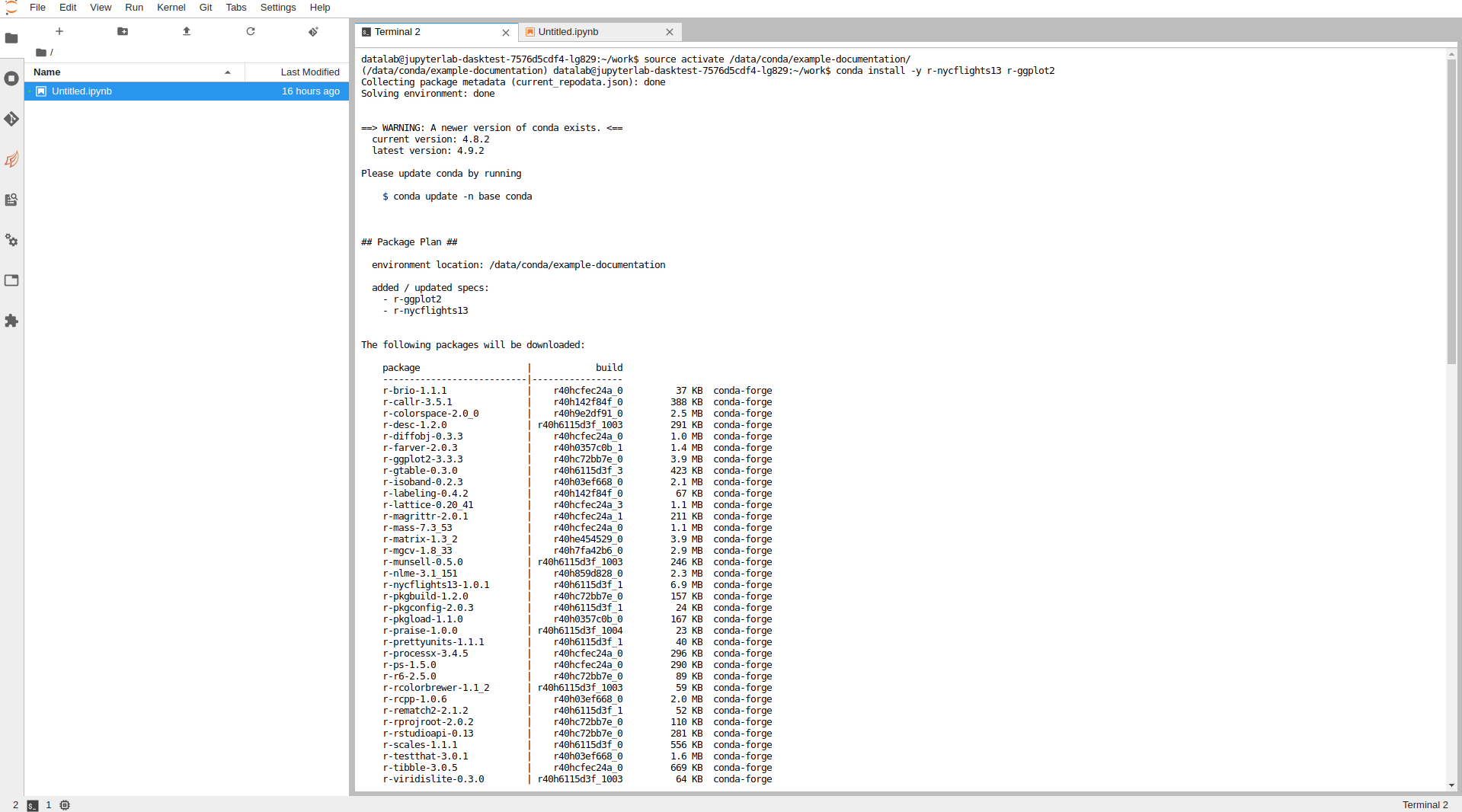
In the case of R conda packages can be installed from a Terminal session, this method differs slightly to the standard way that R packages are installed (generally using commands such as install.packages() from the console, which does also work in most cases.) But this method has advantages as it can install system dependencies as well. Note that when installing R packages from Conda you must prefix the package name with r-.

source activate /data/conda/<environment_name>
conda install -y r-nycflight13 r-ggplot2

3. Example Analysis

Once you have a conda environment set up and some basic packages installed, you can begin to create notebooks and carry out analysis.

Python

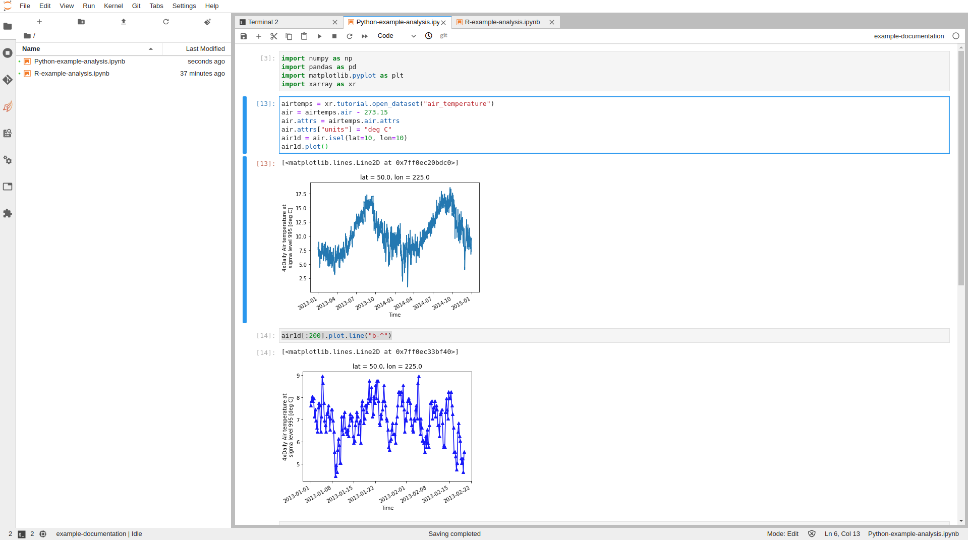
The package xarray includes a number of example datasets that can be used to get used to analysis in Jupyter, below shows a basic example for a simple plot around air temperature.

Paste this code into a Jupyter cell of a python notebook and run the contents (make sure that you have installed the packages in the previous section).

import numpy as np
import pandas as pd
import matplotlib.pyplot as plt
import xarray as xr
# Open air temperature dataset
airtemps = xr.tutorial.open_dataset("air_temperature")
air = airtemps.air - 273.15
air.attrs = airtemps.air.attrs
air.attrs["units"] = "deg C"
air1d = air.isel(lat=10, lon=10)
air1d.plot()
air1d[:200].plot.line("b-^")

R

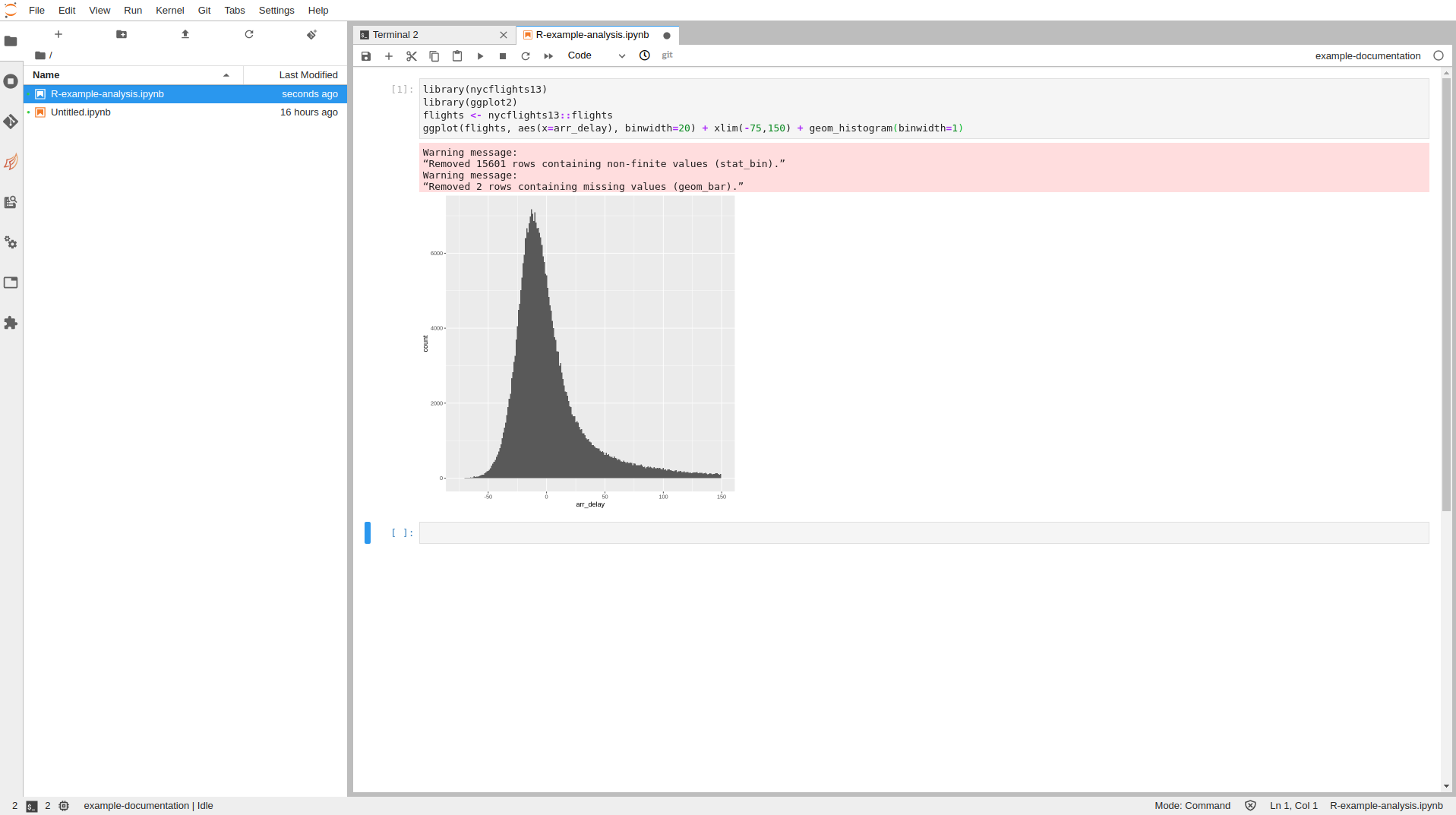
The package nycflights13 contains data relating to flights from a US airport and can be used to get used to handling data within R.

Past the code below into a cell of an R notebook and run the contents (ensure that the packages in the previous section were installed first)

The below simply plots a histogram of the time difference with arrival (negative is early), it represents something looking like a normal distribution.

library(nycflights13)
library(ggplot2)
flights <- nycflights13::flights
ggplot(flights, aes(x=arr_delay), binwidth=20) + xlim(-75,150) + geom_histogram(binwidth=1)

There are a number of very good tutorials which make use of the nycflights13 dataset and help you get started with using a wide arrayy of useful packages and techniques.

8. Conclusion

Congratulations!

In this tutorial, you have:

• Created a new Conda environment within your Jupyter notebook.
• Installed some basic data analysis packages into your Conda environment for both Python and R.
• Ran some example code for Python and R using your Conda environment.

Where next?

You may want to consider these next steps:

• To learn more about Conda environments, visit https://docs.conda.io/projects/conda/en/latest/user-guide/tasks/manage-environments.html.
• To become more familiar with Jupyter, explore the excellent JupyterLab documentation.

My first Datalabs Dask cluster

In this tutorial you will create a Dask cluster within Datalabs, and use it within a notebook.

A Dask cluster created this way can use the same Conda environment as your notebook, and access your project storage.

It is recommended that you should already be familiar with the material in the tutorial My first Jupyter project.

1. What is a Dask cluster?
2. Getting ready
3. Create a Dask cluster
4. Start Dask client
5. Access Dask dashboard
6. Perform Dask calculation
7. Delete Dask cluster
8. Conclusion

1. What is a Dask cluster?

Dask is a flexible library for parallel computing in Python. It works at the scale of a single laptop, enabling parallel processing and extending the size of convenient datasets from "fits in memory" to "fits on disk".

However, it can also work across a cluster of multiple machines. This is probably how you will use it on DataLabs, utilising the compute power of DataLabs.

A Dask cluster consists of:

• A scheduler: this is responsible for deciding how to perform your calculation. It subdivides the work into chunks and co-ordinates how those chunks are performed across a number of workers.
• A number of workers. Workers perform the chunks of calculation that they have been allocated.

In your lab notebook, you will start:

• A Dask client: this is what lets your notebook talk to the scheduler of the Dask cluster, telling the scheduler what calculation you want to perform.
• A Dask dashboard which will give you an indication of how your work is being chunked up, and how your cluster is being utilised.

Further reading:

• Dask: https://docs.dask.org/en/latest/
• Dask clusters: https://distributed.dask.org/en/latest/
• Dask dashboard: https://docs.dask.org/en/latest/diagnostics-distributed.html

2. Getting ready

The Dask workers run Python in a particular environment. If you do not specify a Conda environment for the Dask cluster, then it will run in a default environment. For some situations that will be fine, but in many situations it is less error-prone if the Dask workers and the notebook are using the same environments. This can be achieved by using the same Conda environment in the notebook and the cluster.

This is the approach being taken in this tutorial. Therefore, before proceeding, ensure that you have:

• a project
• project storage
• a JupyterLab notebook
• a Conda environment

If you are unsure how to create these, then please follow the material in the tutorials

• My First Notebook
• My first Jupyter project

3. Create a Dask Cluster

In this section you will create a Dask cluster, in order to use it in your notebook.

Starting point: you should be logged in to DataLabs, in a project you have admin permissions for.

On the left-hand-side, select Dask.

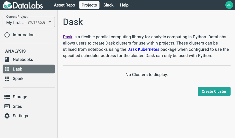
Select Create cluster, and fill out a form to create the Dask cluster.

Note that determining the optimum values for Maximum number of workers, Maximum worker memory and Maximum worker CPU use may require some trial-and-error. If you are simply exploring functionality, it is best to drop these parameters to their minimum values. DataLabs will reserve the memory and CPU for each worker (making those resources unavailable for other users), and will scale the number of workers up from 1 to the maximum (and back down again) depending on the load on the cluster.

Then select Create.

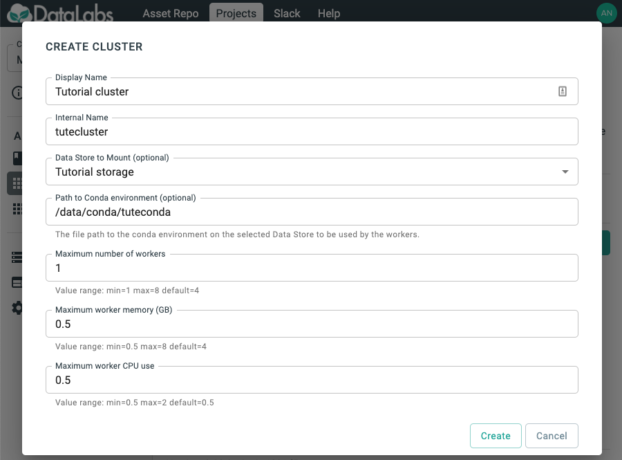
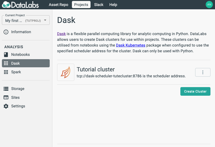
You will then be able to see the cluster that you have created.

4. Start Dask Client

In this section you will start a Dask client, in order to use it to perform distributed calculations.

Starting point: you should be logged in to DataLabs, in a project you have admin permissions for, with a notebook and cluster already created.

On the Dask cluster, select the triple-dot More menu and select Copy snippet. This copies a useful snippet of code that you can use in your notebook.

In your JupyterLab, start a notebook based on the same Conda environment that you used to create your cluster.

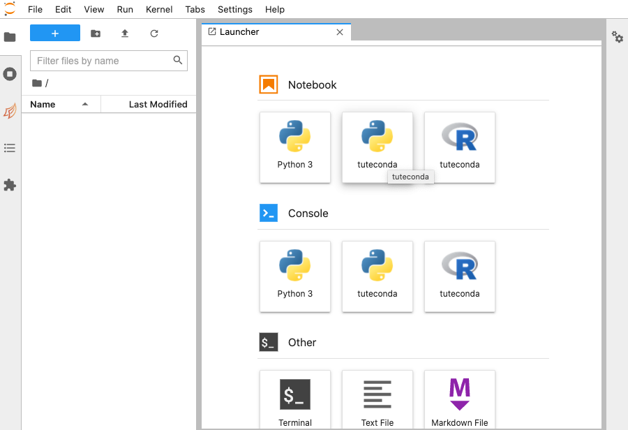
This will ensure that your cluster and your notebook have exactly the same environments.

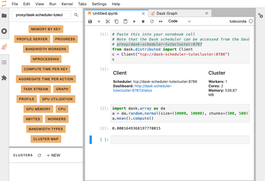
Paste the contents of the clipboard into the notebook cell, and run the notebook.

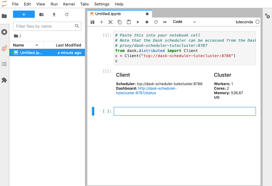
The output shows you that the Client and Cluster are contactable and ready for use.

5. Access Dask Dashboard

In this section you will display the Dask dashboard, in order to see the behaviour of the Dask cluster as it performs calculations.

Starting point: you should be logged in to DataLabs, in a project you have admin permissions for, with a notebook client started from the cluster snippet.

On the left-hand side of the screen is a series of buttons, one of which looks like two orange leaves (the Dask icon). Select the Dask icon to open the Dask JupyterLab extension.

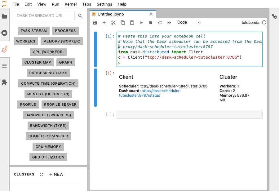
The bottom of the pane gives an alternative way to create Dask clusters. We will not use this, as those Dask clusters do not have access to DataLabs storage, and cannot use a project Conda environment.

However, we can use the extension to access the Dask dashboard. In the pasted snippet text, there is a comment giving the Dask dashboard URL, which starts with proxy/... Copy that address, paste it into the DASK DASHBOARD URL textbox in the Dask JupyterLab extension, and press return. The various dashboard metrics will turn orange, indicating that they are available.

Double-click the GRAPH metric. A new tab appears, showing you that the scheduler is not currently co-ordinating any work.

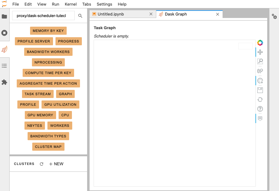
Although less convenient, it is also possible to access the Dask dashboard directly through your browser. Take your notebook URL, e.g.

https://tutproj-tutnb.test-datalabs.nerc.ac.uk/lab

and replace the lab with the Dask dashboard URL starting with proxy/, and then append a final /graph to give

https://tutproj-tutnb.test-datalabs.nerc.ac.uk/proxy/dask-scheduler-tutecluster:8787/graph

This URL gives you direct browser access to the Dask dashboard.

Note that, for security reasons, the cluster and the JupyterLab notebook must reside within the same project.

6. Perform Dask Calculation

In this section you will perform a Dask calculation, observing the cluster behaviour via the Dask dashboard.

Starting point: you should be logged in to DataLabs, with a notebook client and a Dask dashboard.

Copy and paste the following text into the next cell:

import dask.array as da
a = da.random.normal(size=(10000, 10000), chunks=(500, 500))
a.mean().compute()

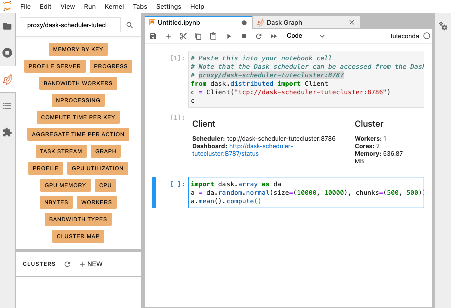
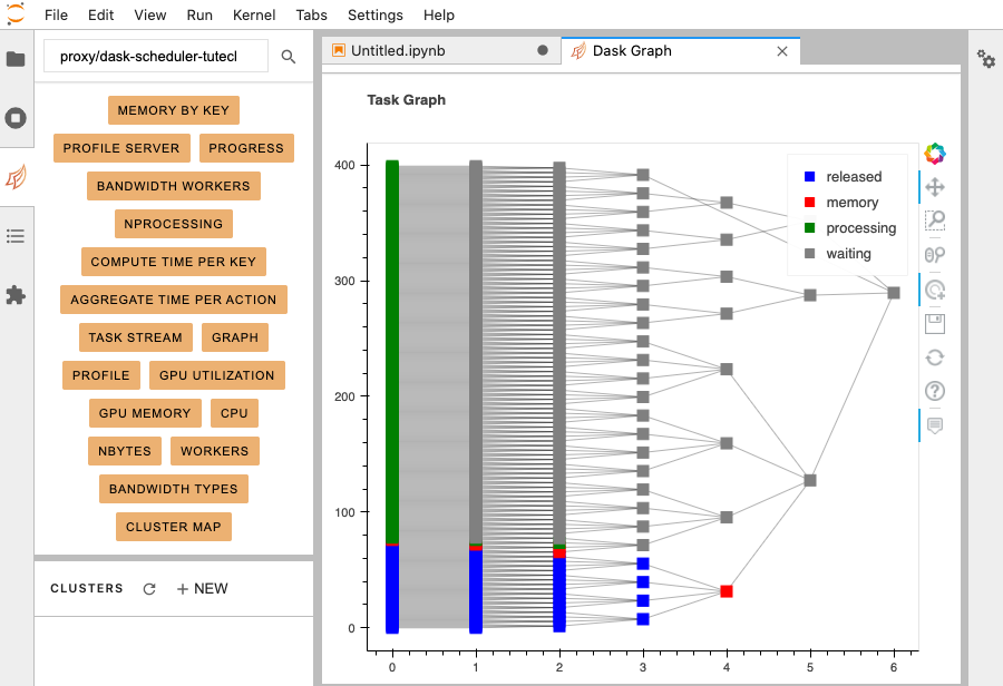
Running this cell will perform the Dask calculation. While the calculation is being performed, you can observe the scheduler co-ordinating the work on the Dask Graph.

Back on the notebook tab, the Dask calculation will be outputted.

7. Delete Dask Cluster

In this section you will delete a Dask cluster, in order to free up resources.

Creating and using clusters is relatively straight-forward and no data is stored in the cluster, so clusters should be deleted when they are no longer required, in order to free up resources for other users.

Starting point: you should be logged in to DataLabs, in a project you have admin permissions for, and a cluster should already exist.

On the Dask cluster, select the triple-dot More menu and select Delete.

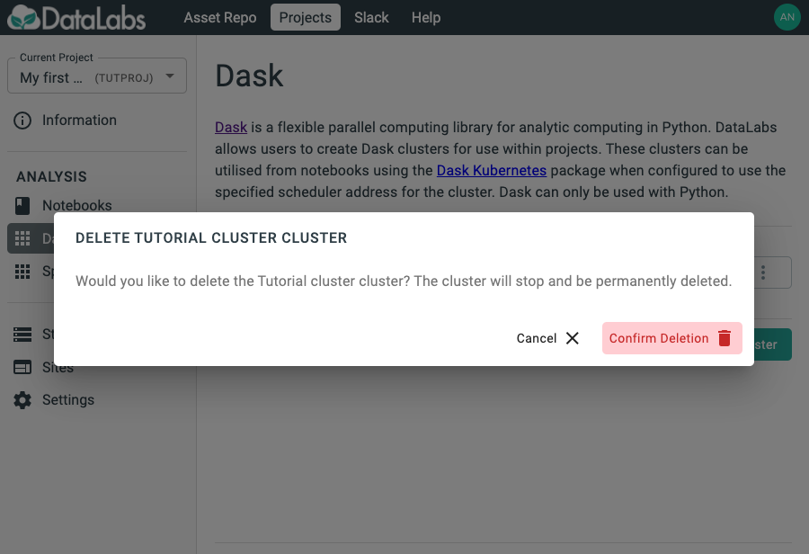
Select Confirm deletion to delete the Dask cluster.

8. Conclusion

Congratulations!

In this tutorial, you have:

• Understood what Dask clusters are.
• Created a Dask cluster, utilising the same Conda environment as your notebook.
• Started the Dask client in a notebook.
• Accessed the Dask dashboard.
• Performed a Dask calculation.
• Deleted the Dask cluster.

It is also possible to access the Data Store from your Dask cluster, just as you would from your notebook; and to create a 'vanilla' Dask cluster, that doesn't require a pre-existing Conda environment.

Where next?

You may want to consider these next steps:

• To learn more about Dask, visit https://docs.dask.org/en/latest/.
• To learn more about Conda package management, visit Managing packages within Conda.

My first Datalabs Spark cluster

In this tutorial, you will create a Spark cluster within Datalabs and use it inside a notebook.

A Spark cluster created this way must use the same Conda environment as your notebook, and requires a project storage.

It is recommended that you should already be familiar with the material in the tutorial My first Jupyter project.

1. What is a Spark cluster?
2. Getting ready
3. Create a Spark cluster
4. Start Spark session
5. Perform Spark calculation (Python)
6. Perform Spark calculation (R)
7. Delete Spark cluster
8. Conclusion

1. What is a Spark cluster?

Spark is a unified analytics engine for large-scale data processing which can be used in both Python and R.

A Spark cluster consists of:

• A scheduler: this is responsible for deciding how to perform your calculation. It subdivides the work into chunks and co-ordinates how those chunks are performed across a number of workers.
• A number of workers. Workers perform the chunks of calculation that they have been allocated.

In your lab notebook, you will start a Spark context or session. This is what lets your notebook talk to the scheduler of the Spark cluster, telling the scheduler what calculation you want to perform.

Further reading:

• Spark: https://spark.apache.org/docs/latest/
• Spark examples: https://spark.apache.org/examples.html

2. Getting ready

The Spark workers run Python in a particular environment.

You must specify a Conda environment for the Spark cluster when it is created. This environment can be created inside a Jupyter notebook.

Before proceeding, ensure that you have:

• a project
• project storage
• a JupyterLab notebook
• a Conda environment

If you are unsure how to create these, then please follow the material in the tutorials

• My First Notebook
• My first Jupyter project

3. Create a Spark Cluster

In this section you will create a Spark cluster, in order to use it in your notebook.

Starting point: you should be logged in to DataLabs, in a project you have admin permissions for. This project should contain a JupyterLab notebook in which you have created a Conda environment.

On the left-hand-side, select Spark.

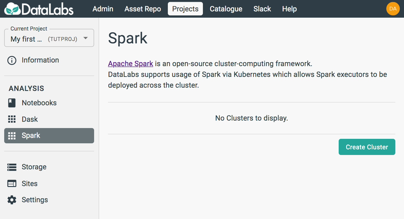
Select Create cluster, and fill out a form to create the Spark cluster.

Note that determining the optimum values for Maximum number of workers, Maximum worker memory and Maximum worker CPU use may require some trial-and-error. If you are simply exploring functionality, it is best to drop these parameters to their minimum values. DataLabs will reserve the memory and CPU for each worker (making those resources unavailable for other users), and will scale the number of workers up from 1 to the maximum (and back down again) depending on the load on the cluster.

Then select Create.

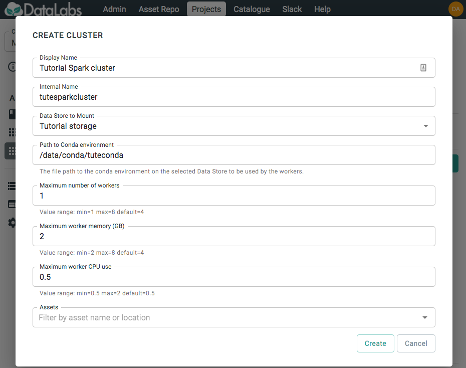
You will then be able to see the cluster that you have created.

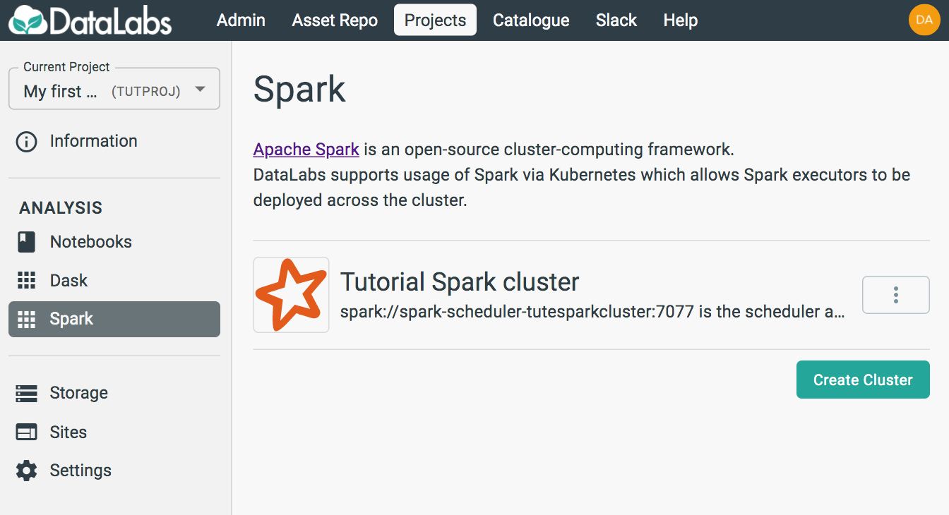
4. Start Spark Session

In this section you will start a Spark session, in order to use it to perform distributed calculations.

Starting point: you should be logged in to DataLabs, in a project you have admin permissions for, with a notebook and Spark cluster already created.

Spark can be used from both Python and R. This section covers how to connect in each language

Python

On the Spark page, find your cluster and select the triple-dot More menu and select Copy Python snippet. This copies a useful snippet of Python code that you can use in your notebook.

In your JupyterLab, start a Python notebook based on the same Conda environment that you used to create your cluster.

Paste the contents of the clipboard into the notebook cell, and run the notebook.

The output shows you that the Spark Cluster is contactable and ready for use.

R

n the Spark page, find your cluster and select the triple-dot More menu and select Copy R snippet. This copies a useful snippet of R code that you can use in your notebook.

In your JupyterLab, start an R notebook based on the same Conda environment that you used to create your cluster.

Paste the contents of the clipboard into the notebook cell, and run the notebook.

Note: You may need to install the SparkR library, if so, you can use the following:

packageurl <- "https://cran.r-project.org/src/contrib/Archive/SparkR/SparkR_3.1.2.tar.gz"
install.packages(packageurl, repos=NULL, type="source")

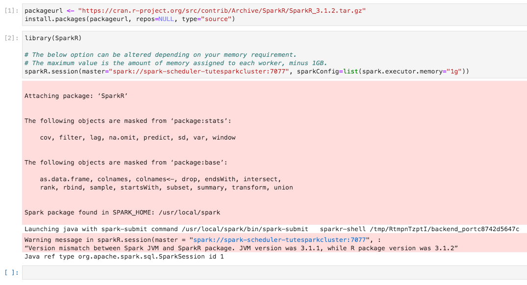
This sets the configuration for the spark "session" so subsequent calls will be made to the specified cluster.

Perform Spark Calculation (Python)

In this section you will perform a Spark calculation using Python.

Starting point: you should be logged in to Datalabs, with a JupyterLab Python notebook connected to a Spark cluster.

The below example is some code that estimates Pi by randomly picking points inside the unit square. The proportion of those points that are also inside the unit circle is approximately pi/4.

Copy and paste the following into the next cell:

import random
NUM_SAMPLES = 100

def inside(p):
    x, y = random.random(), random.random()
    return x*x + y*y < 1

count = sc.parallelize(range(0, NUM_SAMPLES)) \
             .filter(inside).count()
print("Pi is roughly %f" % (4.0 * count / NUM_SAMPLES))

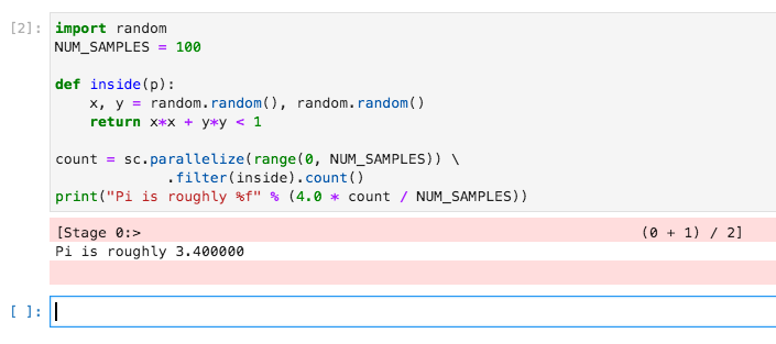
To clear up resources, you can run the following to stop the context:

sc.stop()

Perform Spark Calculation (R)

In this section you will perform a Spark calculation using R.

Starting point: you should be logged in to Datalabs, with a JupyterLab R notebook connected to a Spark cluster.

The below example is some code that estimates Pi by randomly picking points inside the unit square. The proportion of those points that are also inside the unit circle is approximately pi/4.

Copy and paste the following into the next cell:

inside <- function(p) {
  x <- runif(1)
  y <- runif(1)
  return(x*x + y*y < 1)
}

NUM_SAMPLES <- 100
l <- spark.lapply(seq(0, NUM_SAMPLES-1), inside)
count <- length(Filter(isTRUE, l))
pi <- (4 * count) / NUM_SAMPLES
sprintf(fmt="Pi is roughly %f", pi)

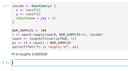
To clear up resources, you can run the following to stop the session:

sparkR.stop()

7. Delete Spark Cluster

In this section you will delete a Spark cluster, in order to free up resources.

Creating and using clusters is relatively straight-forward and no data is stored in the cluster, so clusters should be deleted when they are no longer required, in order to free up resources for other users.

Starting point: you should be logged in to DataLabs, in a project you have admin permissions for, and a cluster should already exist.

On the Spark cluster, select the triple-dot More menu and select Delete.

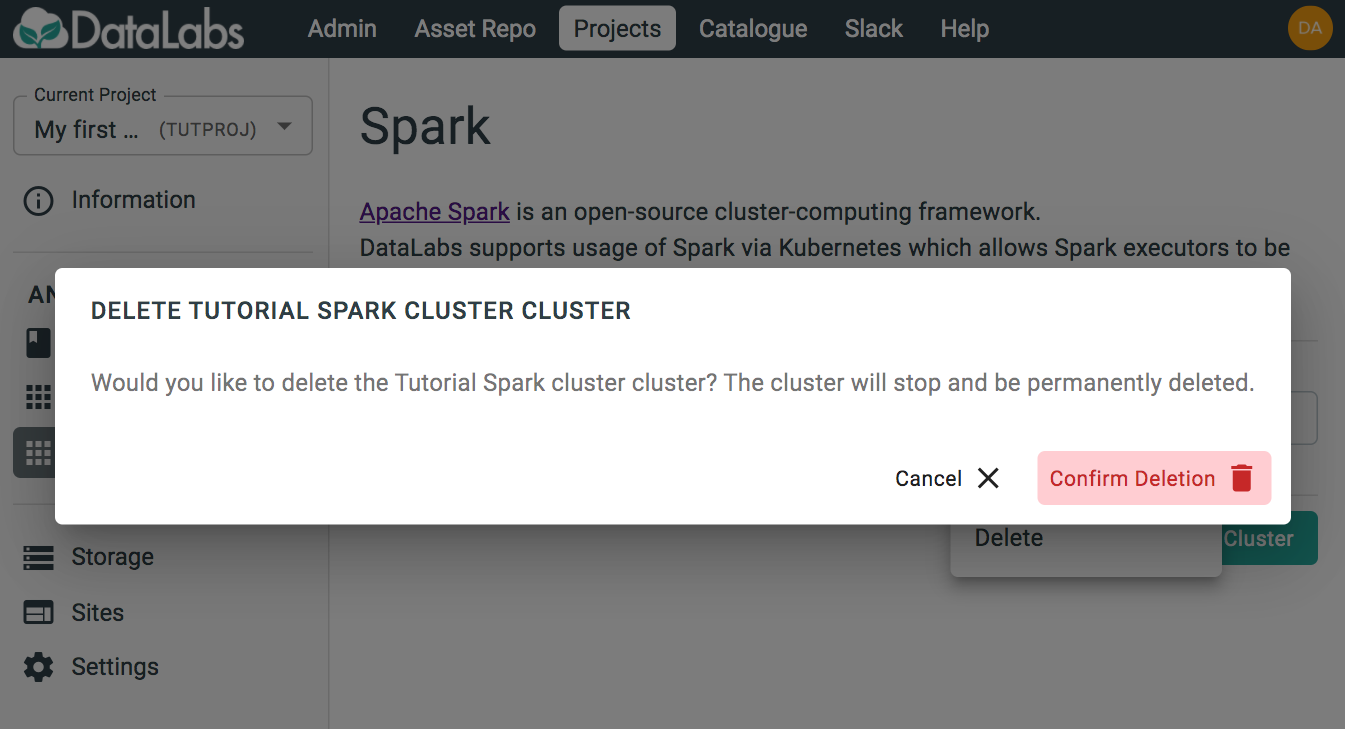
Select Confirm deletion to delete the Spark cluster.

8. Conclusion

Congratulations!

In this tutorial, you have:

• Understood what Spark clusters are.
• Created a Spark cluster, utilising the same Conda environment as your notebook.
• Started a Spark context in a Python notebook.
• Started a Spark session in an R notebook.
• Performed Spark calculations in Python and R.
• Deleted the Spark cluster.

Where next?

You may want to consider these next steps:

• To learn more about Spark, visit https://spark.apache.org/docs/latest/
• To learn more about Conda package management, visit Managing packages within Conda.

My first Panel Site

In this tutorial you will create a Panel site within Datalabs, allowing you to visualise and interact with a notebook.

1. Getting ready
2. Create a Panel site
3. Launch Panel
4. Delete Panel site
5. Conclusion

1. Getting Ready

A Panel site can be used to visualise a Jupyter notebook, so, before continuing, you will need the following:

• A project
• Project storage
• A JupyterLab notebook
• (Optionally) A Conda environment

For tutorials on the above, see:

• My First Notebook
• My first Jupyter project

An example notebook might contain the following:

import matplotlib.pyplot as plt
import panel as pn

pn.extension()
fig = plt.figure()

%matplotlib inline

xs = []
ys = []

int_slider = pn.widgets.IntSlider(name='X value', start=-10, end=10, step=1, value=3)

@pn.depends(int_slider.param.value)
def get_plot(x):
    y = x ** 2

    if x not in xs:
        xs.append(x)
        ys.append(y)

    plt.clf()
    plt.plot(xs, ys, 'ro', markersize=5)
    plt.plot(x, y, 'go', markersize=10)

    return fig

dashboard = pn.Row(
    pn.Column("My Chart", int_slider),
    get_plot # plot function
)

dashboard.servable()

This code will produce a simple dashboard with a slider that chooses the x value for a plot showing the x^2 function.

2. Create a Panel site

In this section you will create a Panel site.

Starting point: you should be logged in to DataLabs, in a project you have admin permissions for. This project should contain a JupyterLab notebook containing the code you want to host with Panel.

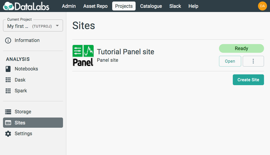
On the left-hand side, select Sites.

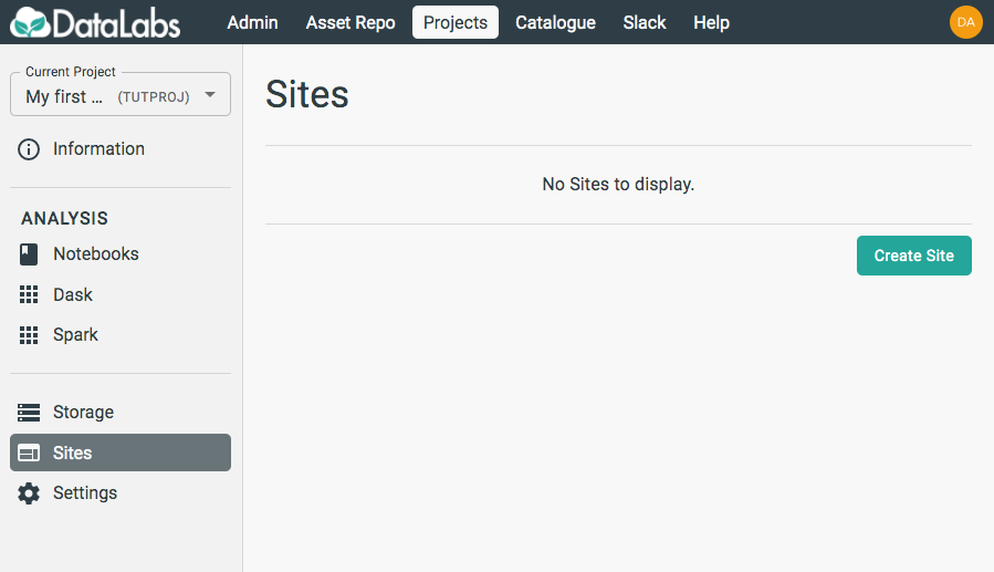
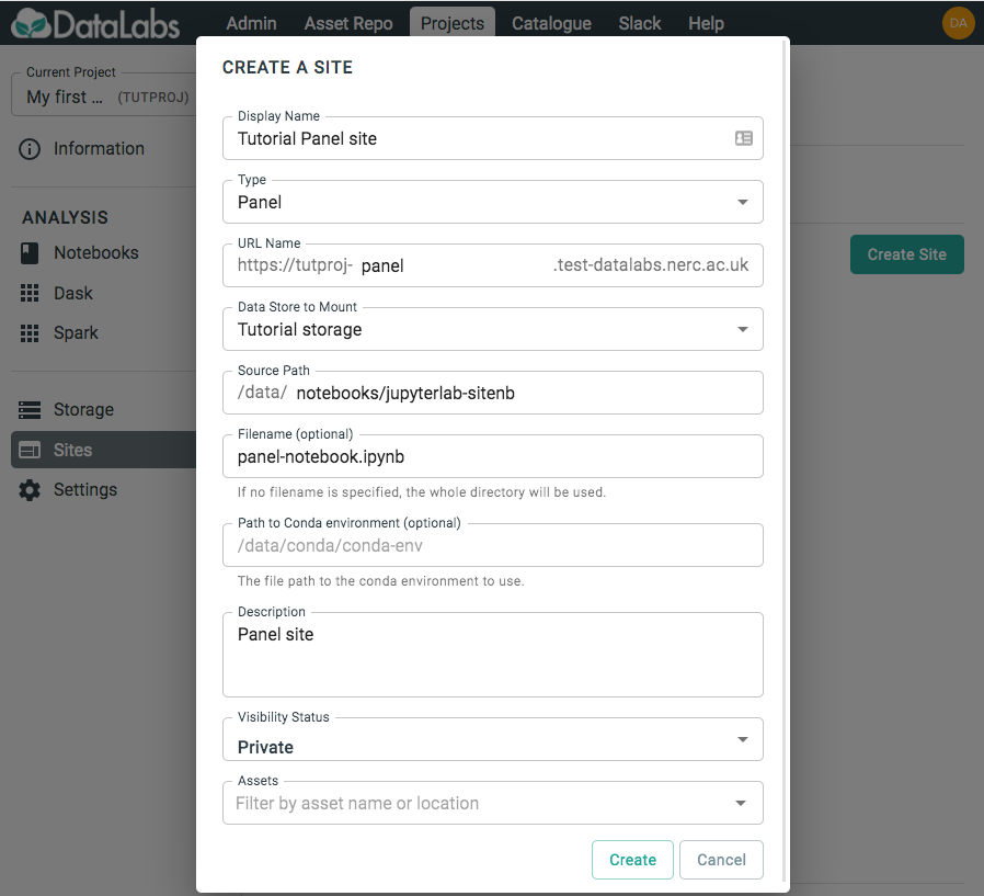
Select Create Site and fill out the form. In this form, the Source Path should point to where your notebook code exists within your Project Storage, for example /data/notebooks/jupyterlab-notebook.

By default, the Panel site will host all notebook files in the Source Path directory, providing a landing page to choose which one to view. You also have the option of choosing a specific file to host, meaning that the site will only display that notebook. The site will still be able to access other files in the directory if necessary, such as data files and scripts.

In addition, you can choose a Conda environment to use for the kernel when the notebook(s) is run on the site, allowing for the use of packages in that Conda environment. This environment is chosen at the top level, and Panel sites do not support multiple kernels for different notebooks in the case that all notebooks in the Source Path are displayed.

When happy with the settings, click Create.

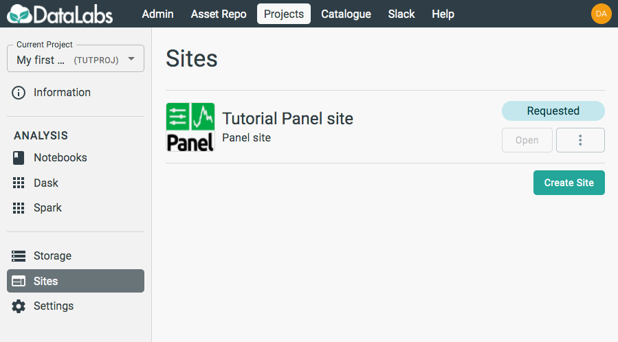
Once created, you will be able to see your Site appear in the list, and its status will change from Requested to Ready once it is available to launch.

3. Launch Panel

In this section you will launch a Panel site.

Starting point: you should be logged in to DataLabs, in a project you have at least viewer permissions for. This project should contain a Panel site connected to a JupyterLab notebook.

On the left-hand side, select Sites.

On this page, you should see any Sites you have access to view. Click on Open on your Panel site.

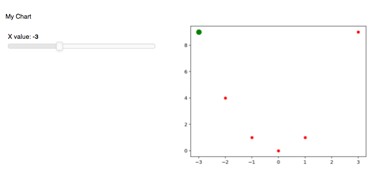
If the site was created with a specific notebook file, then the launched page might look something like the above image. In this case, we have an interactive slider which is the output of a cell in the notebook that is being hosted.

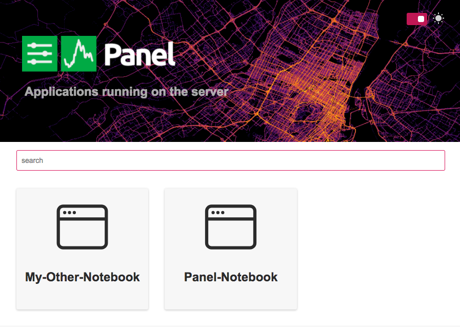
If the site was created without a specific file, then all notebooks in the chosen directory will be available to view. The default landing page looks something like the above image, and selecting a notebook will launch it.

4. Delete Panel site

In this section you will delete a Panel site.

As sites are driven by the contents of a notebook and doesn't contain the code itself, they can be deleted when they are no longer needed.

Starting point: you should be logged in to DataLabs, in a project you have admin permissions for, and a Panel site should already exist.

On the Panel site, select the triple-dot More menu and select Delete.

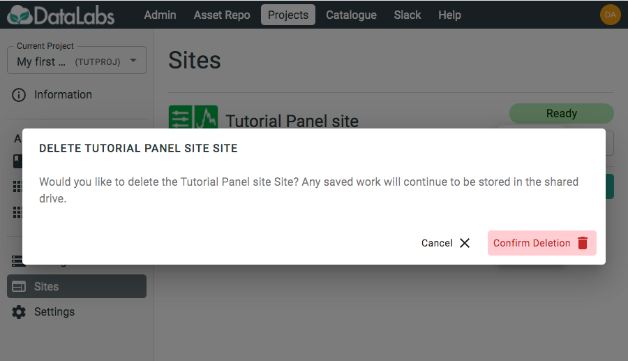
Select Confirm deletion to delete the Panel site.

5. Conclusion

Congratulations!

In this tutorial, you have:

• Created a Panel site linked to a notebook.
• Launched the site and used its interactive elements.
• Deleted the Panel site.

Where next?

To learn more about Panel, visit https://panel.holoviz.org/getting_started/

My first Voilà Site

In this tutorial you will create a Voilà site within Datalabs, allowing you to visualise and interact with a notebook.

1. Getting ready
2. Create a Voilà site
3. Launch Voilà
4. Delete Voilà site
5. Conclusion

1. Getting Ready

A Voilà site can be used to visualise a Jupyter notebook, so, before continuing, you will need the following:

• A project
• Project storage
• A JupyterLab notebook
• (Optionally) A Conda environment

For tutorials on the above, see:

• My First Notebook
• My first Jupyter project

An example notebook might contain the following in a cell:

import ipywidgets as widgets

slider = widgets.FloatSlider(description='$x$')
text = widgets.FloatText(disabled=True, description='$x^2$')

def compute(*ignore):
    text.value = str(slider.value ** 2)

slider.observe(compute, 'value')

slider.value = 4

widgets.VBox([slider, text])

Note that this example requires the ipywidgets package to be installed in the Conda environment if that is being used to run the notebook.

2. Create a Voilà site

In this section you will create a Voilà site.

Starting point: you should be logged in to DataLabs, in a project you have admin permissions for. This project should contain a JupyterLab notebook containing the code you want to host with Voilà.

On the left-hand side, select Sites.

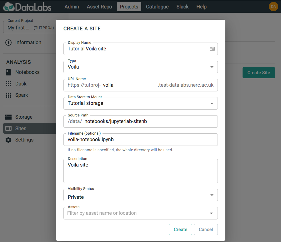
Select Create Site and fill out the form. In this form, the Source Path should point to where your notebook code exists within your Project Storage, for example /data/notebooks/jupyterlab-notebook.

By default, the Voilà site will host all notebook files in the Source Path directory, providing a landing page to choose which one to view. You also have the option of choosing a specific file to host, meaning that the site will only display that notebook. The site will still be able to access other files in the directory if necessary, such as data files and scripts.

Note that Voilà sites will automatically pick up and use the kernel associated with the select notebook. So, if a particular notebook requires a Conda environment, it will use this.

When happy with the settings, click Create.

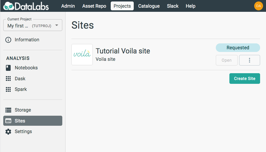
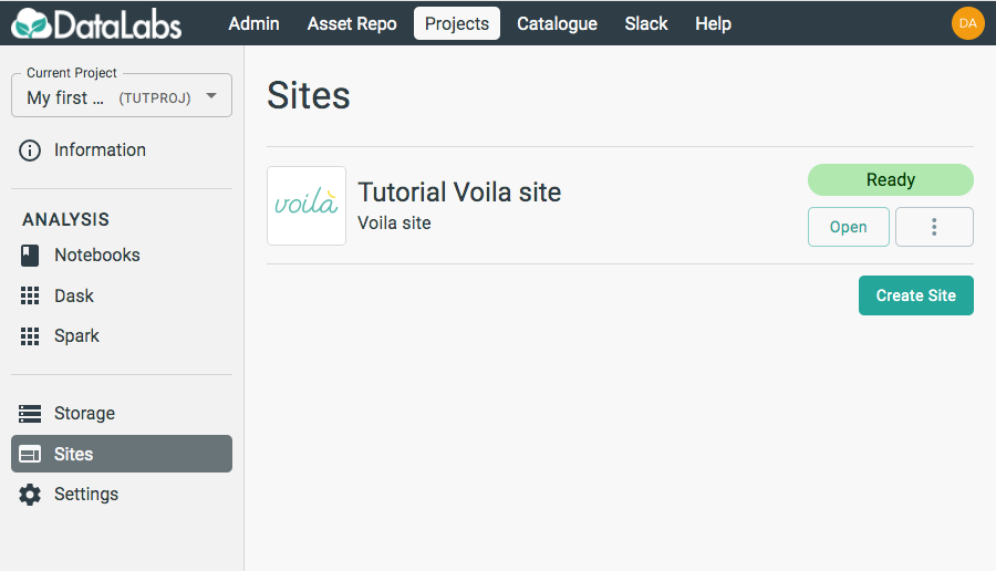
Once created, you will be able to see your Site appear in the list, and its status will change from Requested to Ready once it is available to launch.

3. Launch Voilà

In this section you will launch a Voilà site.

Starting point: you should be logged in to DataLabs, in a project you have at least viewer permissions for. This project should contain a Voilà site connected to a JupyterLab notebook.

On the left-hand side, select Sites.

On this page, you should see any Sites you have access to view. Click on Open on your Voilà site.

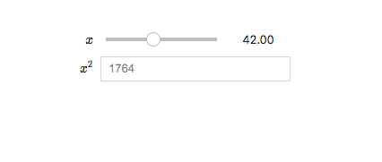
If the site was created with a specific notebook file, then the launched page might look something like the above image. In this case, we have an interactive slider which is the output of a cell in the notebook that is being hosted.

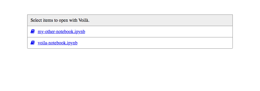
If the site was created without a specific file, then all notebooks in the chosen directory will be available to view. The default landing page looks something like the above image, and selecting a notebook will launch it.

4. Delete Voilà site

In this section you will delete a Voilà site.

As sites are driven by the contents of a notebook and doesn't contain the code itself, they can be deleted when they are no longer needed.

Starting point: you should be logged in to DataLabs, in a project you have admin permissions for, and a Voilà site should already exist.

On the Voilà site, select the triple-dot More menu and select Delete.

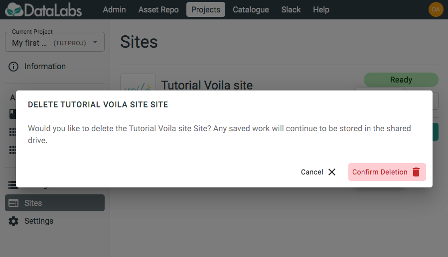
Select Confirm deletion to delete the Voilà site.

5. Conclusion

Congratulations!

In this tutorial, you have:

• Created a Voilà site linked to a notebook.
• Launched the site and used its interactive elements.
• Deleted the Voilà site.

Where next?

To learn more about Voilà, visit https://github.com/voila-dashboards/voila

My first Streamlit Site

In this tutorial you will create a Streamlit site within Datalabs, allowing you to produce visualisations and interactable elements from your code.

1. Getting ready
2. Create a Streamlit site
3. Launch, edit and delete a Streamlit site
4. Conclusion

Getting ready

Streamlit is a tool to turn data analysis scripts into web apps. To use it in DataLabs, you will need the following:

• A project
• A data store
• A Conda environment
• A notebook or web IDE to edit code in the project storage (e.g JupyterLab or Visual Studio Code)

You can see tutorials to get started at:

• My First Notebook
• My first Jupyter project
• My first Visual Studio Code project
• Conda Environments Quick-Start-Guide

You'll need to have Streamlit installed in your Conda environment, so if you haven't already, run

conda install streamlit

to get it installed.

Create a Streamlit site

Streamlit doesn't have built-in support for Jupyter notebooks, so you need to create a .py file to be the entry point for the app. You'll have to be logged into DataLabs. We'll assume you have already saved your Streamlit app into a file named app.py in your storage, and installed Streamlit into a Conda environment called my-env.

In your project, navigate to Sites:

Choose Create Site and fill out the form. Set Source Path to the directory containing your Streamlit file, such as /data/notebooks/jupyterlab-notebook, and set Filename to the name of the file itself, such as app.py. Also set the Conda environment path to point to the environment with Streamlit installed, in this example /data/conda/my-env.

Once the environment and storage are set up, the Streamlit app runs in the same Conda environment as any notebooks using that environment, and has filesystem access to the whole store. This means that it can access any data files and assets that are present in the store.

Launch, edit and delete a Streamlit site

Once a site has been created, it can be viewed, edited and opened from the Sites page:

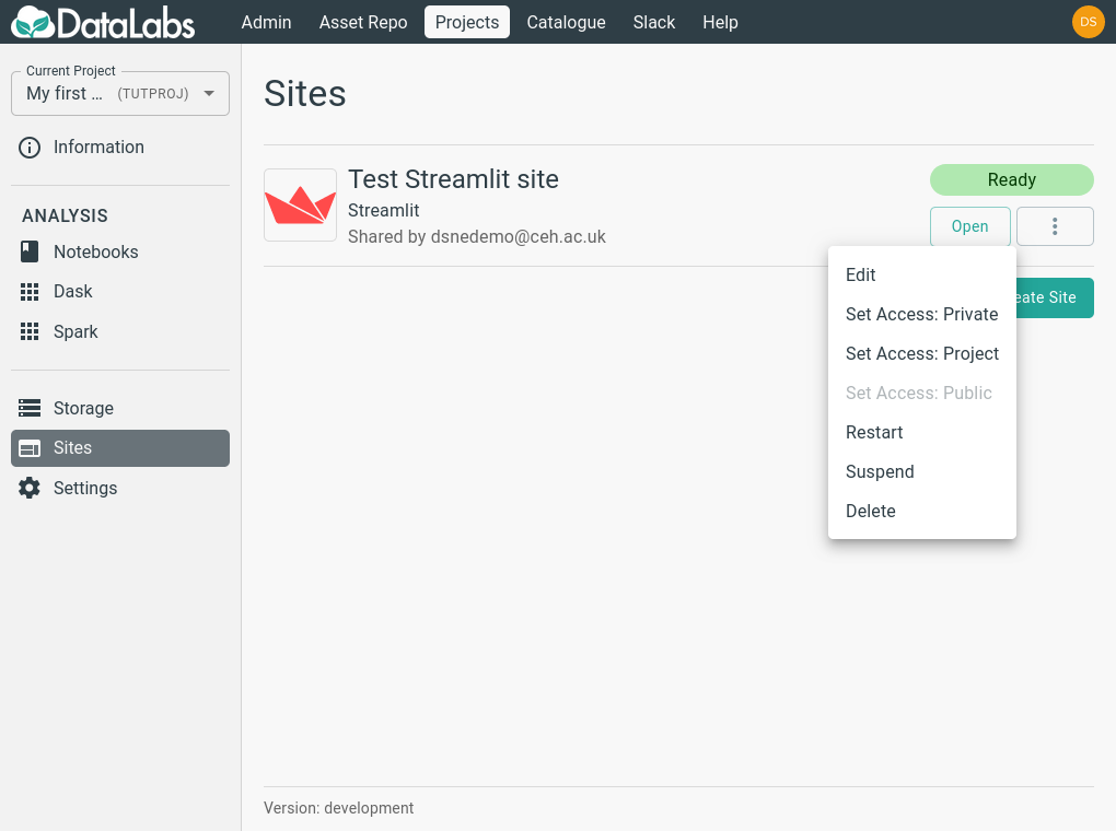
Due to technical limitations in the DataLabs platform, Streamlit apps do not automatically update when changes are made to the underlying Python file.

To see the results of editing your site, you need to restart the site by clicking the Restart button.

Streamlit sites contain no data or state that is not stored on the associated storage, so when no longer needed, it is safe to delete it by pressing the Delete button.

Conclusion

Congratulations!

In this tutorial, you should have learned how to create a Streamlit site, view and interact with it, edit its settings and delete it.

Where next?

For more information about Streamlit, see its homepage at https://streamlit.io/.

My first Shiny Site

In this tutorial you will create a Shiny site within Datalabs, allowing you to visualise and interact with a notebook.

1. Getting ready
2. Create a Shiny site
3. Launch Shiny
4. Delete Shiny site
5. Conclusion

1. Getting Ready

Shiny is an open source R package that provides an elegant and powerful web framework for building web applications using R. Before continuing, you will need the following:

• A project
• Project storage
• A RStudio Notebook

For tutorials on the above, see:

• My First Notebook
• My first RStudio project

This code will produce a simple dashboard with some controls that change a scatter plot.

2. Create a Shiny site

In this section you will create a Shiny site.

Starting point: you should be logged in to DataLabs, in a project you have admin permissions for. This project should contain a blank RStudio notebook.

In order to begin, open your RStudio notebook and create a new project ensuring to select "Shiny". This will trigger some actions like initialising renv and may take a few minutes.

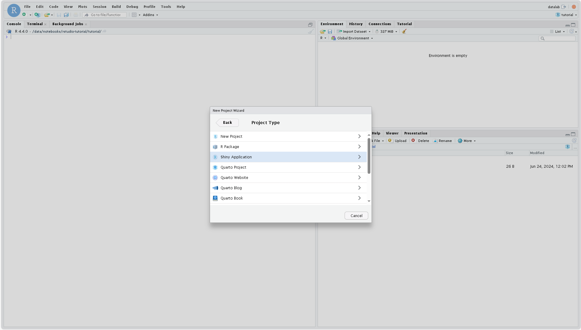
NOTE: When working on more advanced Shiny sites that use custom packages, you should always enable renv when you create the RStudio project. This will track all dependencies used in the project, and they can be loaded by the Shiny site once it has been created by initialising renv in the Shiny code itself. While this isn't required for this minimal example, generally it's advisable to work this way.

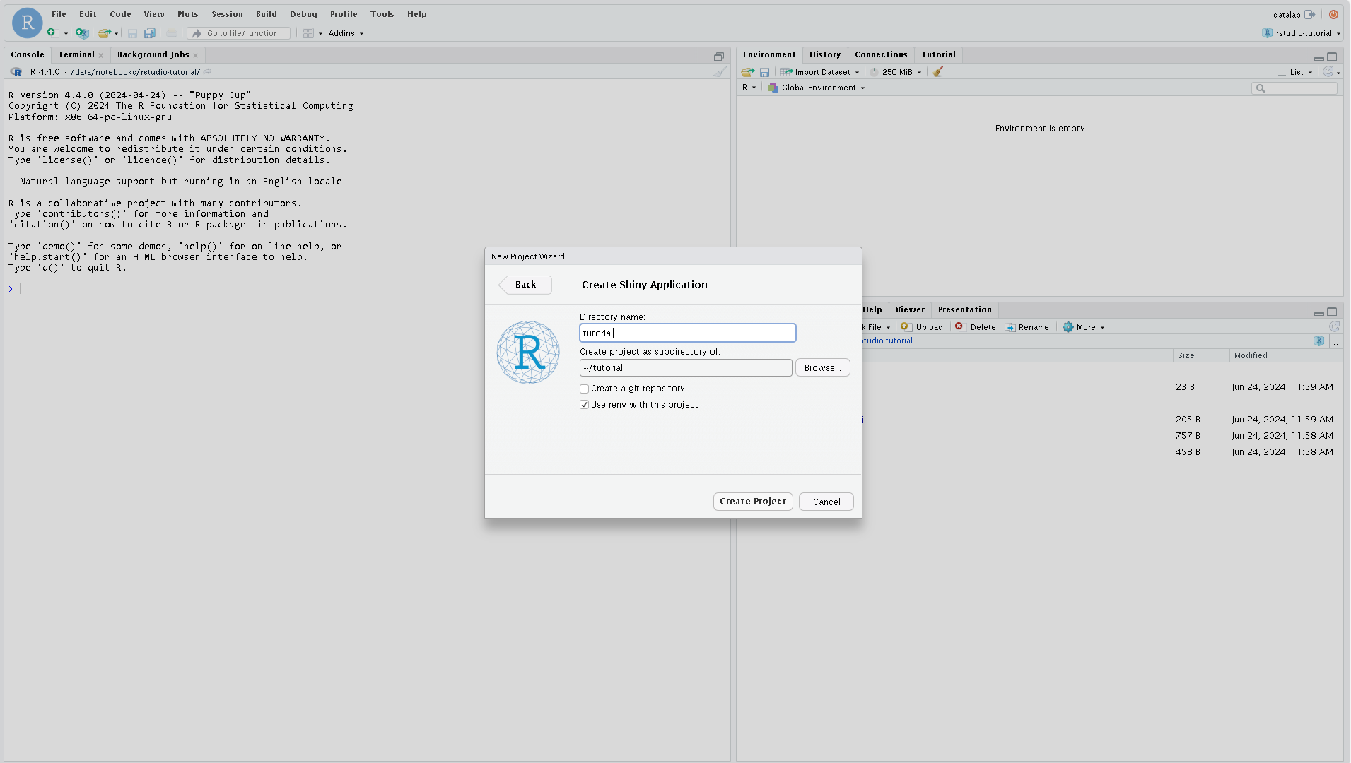
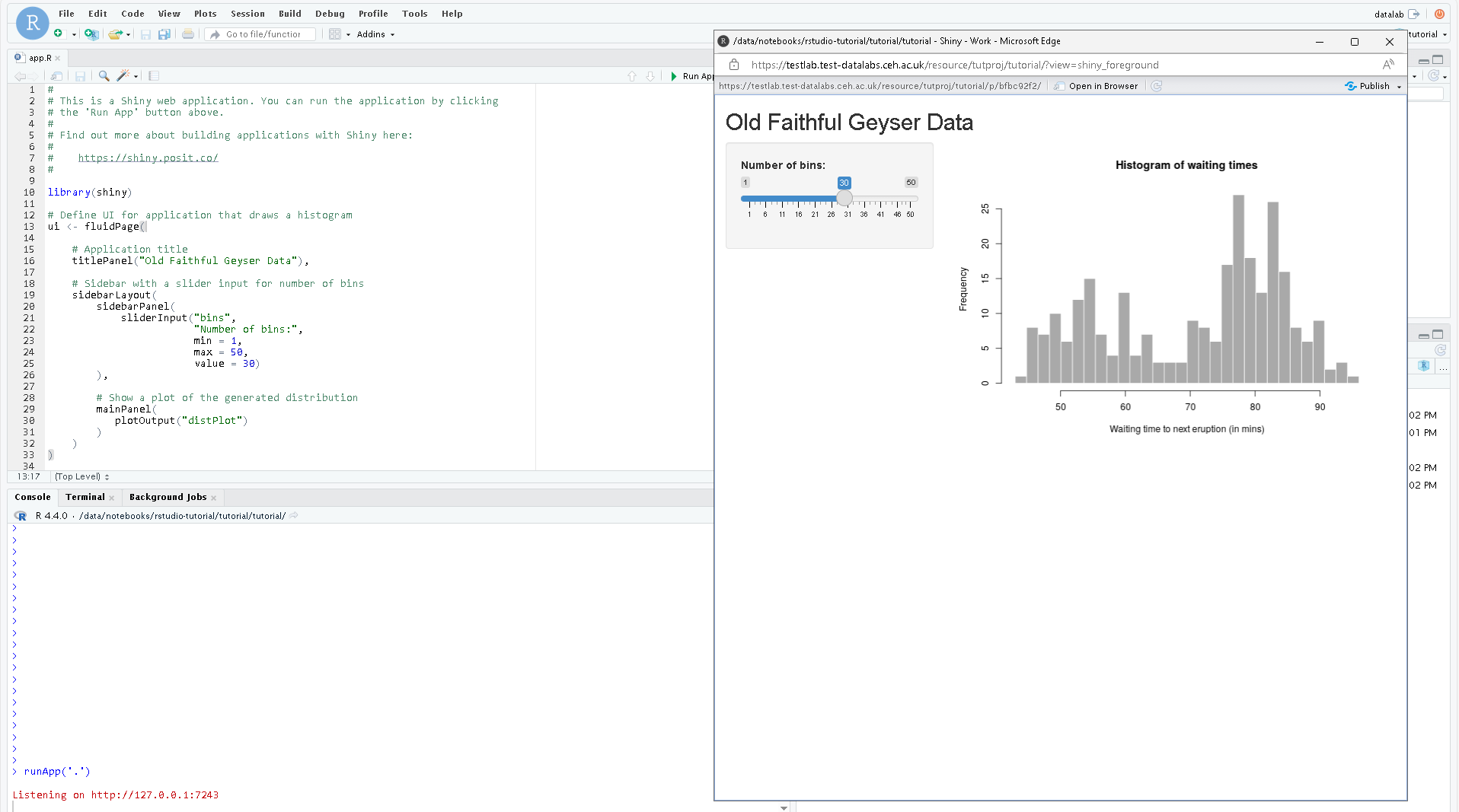
Once complete, this should have generated a new folder with an existing app.R file in which serves as a good example on how to work with Shiny.

Next from DataLabs, on the left-hand side, select Sites.

Select Create Site and fill out the form. In this form, the Source Path should point to where your app.R code exists within your Project Storage, for example /data/notebooks/rstudio-notebook/tutorial. (Assuming the project created in RStudio was called tutorial).

When creating a site you can select a visibility status depending on the target audience. These are as follows;

• Private - This option should be chosen when working alone with no need to share access to the site.
• Project - When you wish to share access to the site with others within the project in which you are working.
• Public - If you wish there to be no authentication in place - allowing you to share access with the site with anyone on the internet.

Note that if you wish to change the visibility status after the notebook this is also possible.

At this stage it is also possible to attach assets to your site, see this page for further information.

By default, the Shiny site will look for app.R or main.R/server.R. If nothing is present it will simply show a blank index page. The site will still be able to access other files in the directory if necessary, such as data files and scripts.

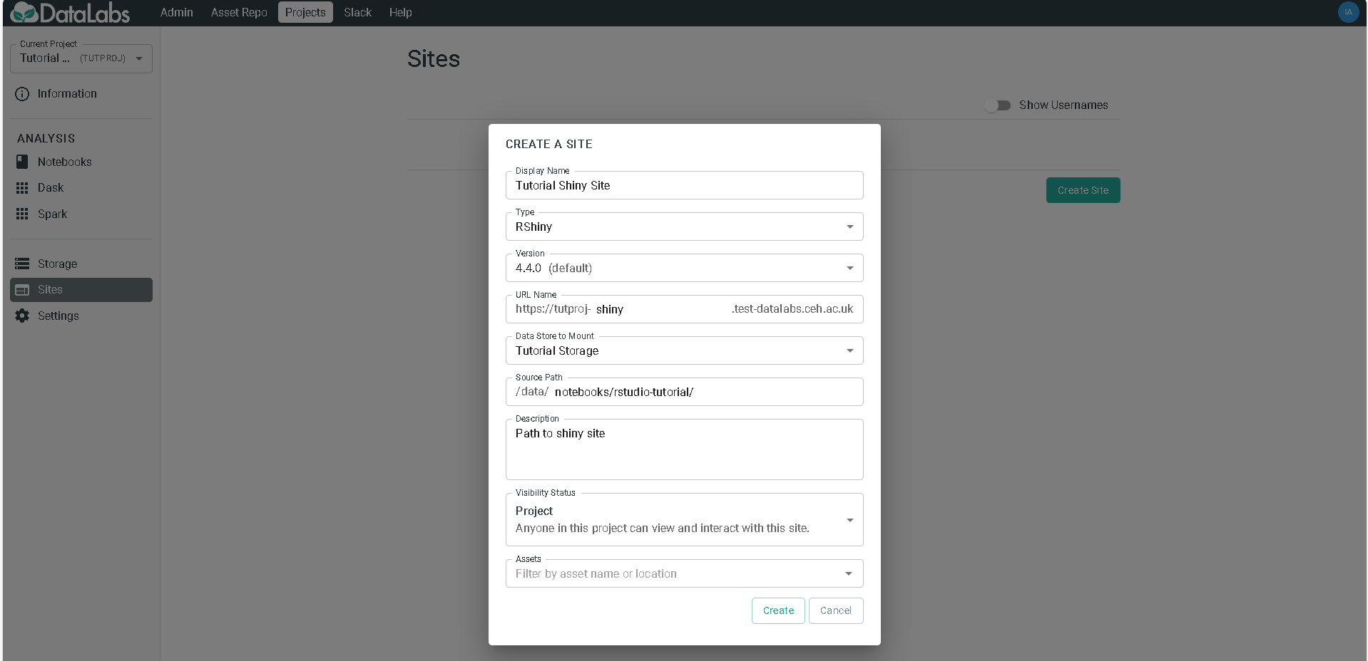
When happy with the settings, click Create.

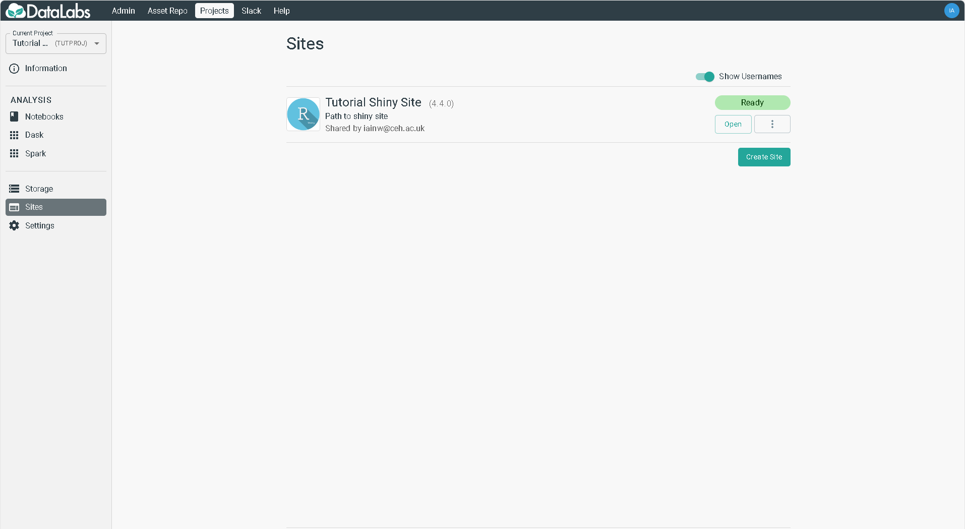
Once created, you will be able to see your Site appear in the list, and its status will change from Requested to Ready once it is available to launch.

3. Launch Shiny

In this section you will launch a Shiny site.

Starting point: you should be logged in to DataLabs, in a project you have at least viewer permissions for. This project should contain a Shiny site connected to a RStudio notebook.

On the left-hand side, select Sites.

Click on Open on your Shiny site.

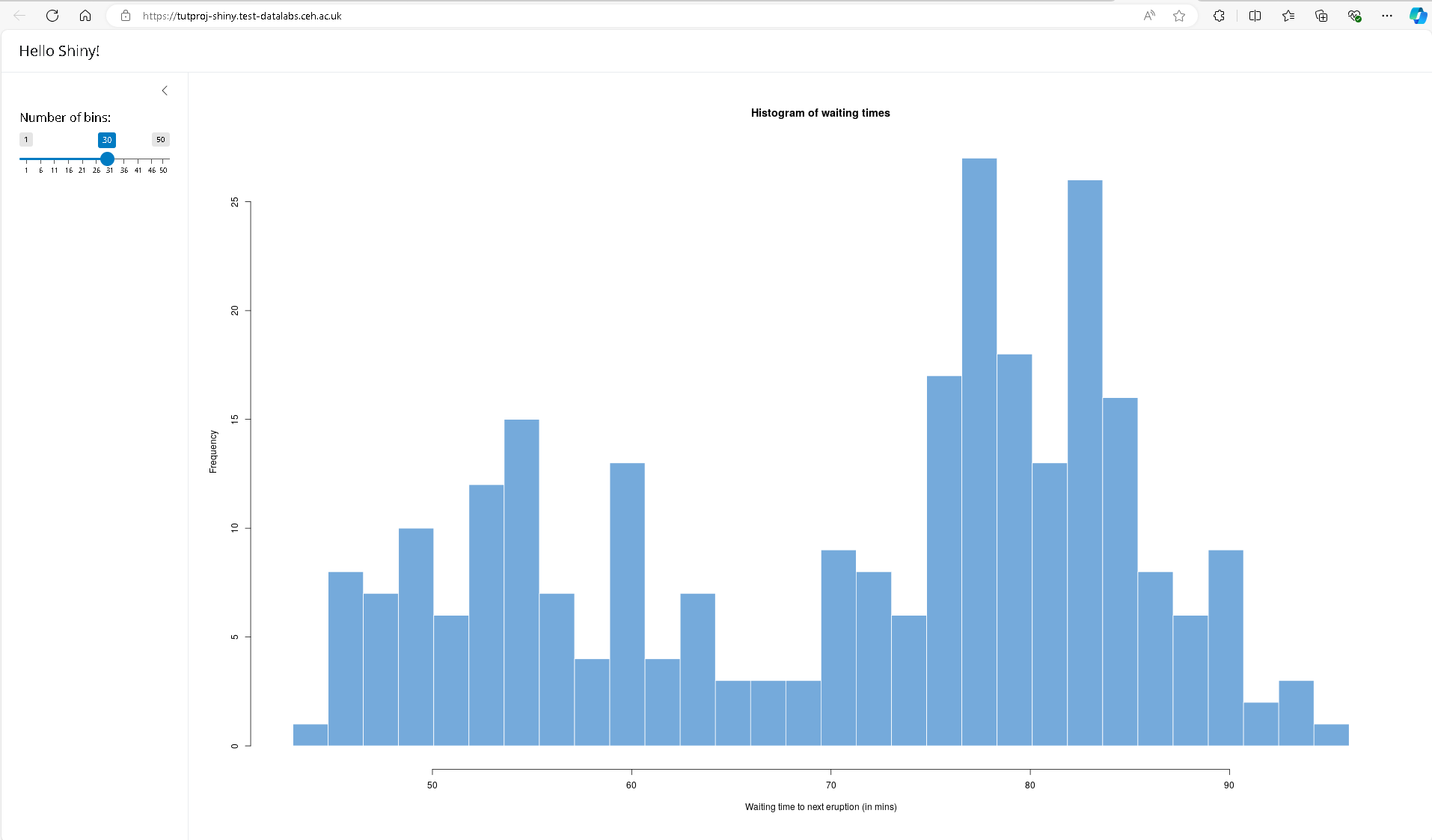
You should be able to see the default Shiny example histogram successfully loaded.

4. Delete Shiny site

In this section you will delete a Shiny site.

As sites are driven by the contents of a notebook and doesn't contain the code itself, they can be deleted when they are no longer needed.

Starting point: you should be logged in to DataLabs, in a project you have admin permissions for, and a Shiny site should already exist.

On the Shiny site, select the triple-dot More menu and select Delete.

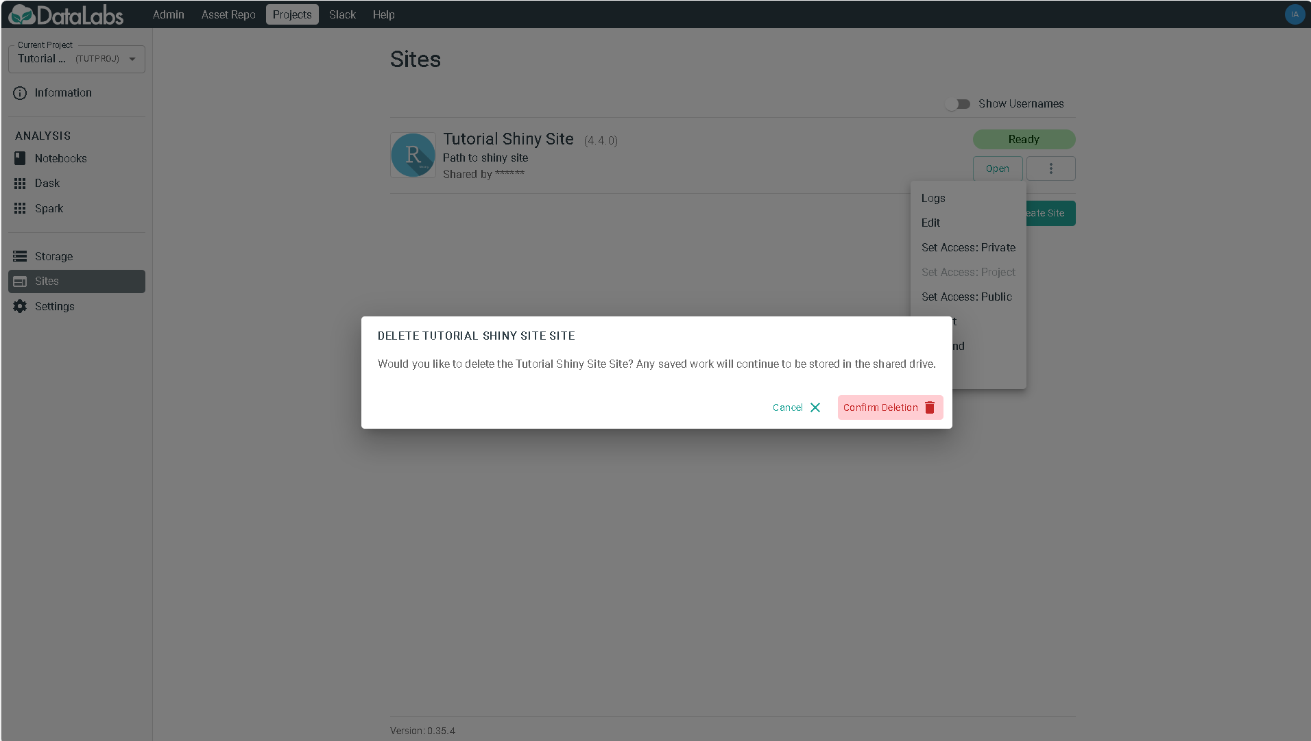
Select Confirm deletion to delete the Shiny site.

5. Conclusion

Congratulations!

In this tutorial, you have:

• Created a Shiny site linked to a notebook.
• Launched the site and used its interactive elements.
• Deleted the Shiny site.

Where next?

To learn more about Shiny, visit https://shiny.posit.co/

Dependency management with Packrat

Packrat is a dependency management system for R developed by RStudio. This provides an isolated, portable and reproducible R environment for each project. Packrat is included by default in the notebooks offered within Datalabs (Jupyter and Zeppelin). Below is a quick summary regarding the use of packrat in the datalabs environment, further information about this package can be found here.

Quick-start guide

Initialising a new project

To use Packrat to manage the R libraries for a project first set the working directory and run the packrat::init command. This initialisation step is only required to be run once to set-up a private library to store the libraries required for the project.

setwd('/data/example_project')
packrat::init()

Opening a Packrat managed project

Once initialised, a project can be opened using the packrat::on function. This will set the private project library for installing and opening of packages. The default global library can be restored by running the packrat::off command. When using Spark the clean.search.path = FALSE argument should be given to the on function, this prevents unloading the SparkR library (see here for more information).

setwd('/data/example_project')
packrat::on()

Installing a package

An R package can be installed in the private project library using the base install.packages function. The project lockfile (used to restore libraries) can then be updated by running packrat::snapshot.

install.packages('fortunes')
packrat::snapshot()

Installing a package specific version

Packrat can additionally manage packages installed via the devtools library. This allows for the installation of specific package versions from CRAN and development versions from GitHub.

# From CRAN
devtools::install_version('zoo', version='1.7-14')
packrat::snapshot()

# From GitHub - userName/repoName@version
devtools::install_github('IRkernel/IRkernel@0.8.8')
packrat::snapshot()

Removing a package

Packaged that are no longer required can be deleted using the remove.packages function, this will remove the package from the private project library. The project lockfile can then be updated using the packrat::snapshot command.

remove.packages('fortunes')
packrat::snapshot()

Restore project packages

The R dependencies managed by packrat are recorded in a lockfile, this includes details on the source and version of the installed packages. When calling packrat::restore the project library is updated to reflect the lockfile. This can be used to maintain a exact copy of your working R set-up and can be included with version control.

This functionality is especially useful within DataLabs when using a project on an alternative notebook type or when needing a library within Spark. For more information see here.

packrat::restore()

Dependency management with Conda on Jupyter

When using Datalabs the recommended way to install packages is through use of Conda. This is a flexible package/library management tool that can be used to install dependencies across multiple languages and platforms (for more information see https://docs.conda.io/en/latest/).

One of the key advantages of Conda is allowing dependencies (including, but not limited packages, binaries & libraries) to be captured alongside project code. It is the default package manager for Jupyter Notebooks. Conda Environments utilize Conda to allow users to setup isolated sets of dependencies. This offers numerous advantages, but practically for DataLabs this allows dependencies to be used within multiple notebooks and persisted when notebooks are rescheduled across the Kubernetes cluster.

Quick-start guide

In order for Conda environments to be persisted within DataLabs, they must be stored on the /data mount point which is shared among notebooks of the same project. Some wrapper commands have been written to make this easier, but users are free to look at Conda Documentation themselves.

Initialising a new project

A Conda environment can be setup by opening a Jupyter notebook/lab and from the terminal running the following command.

env-control add new-environment

This will trigger the creation of a Conda environment as well as adding Jupyter Kernels for both R & Python by default which are persisted on the data volume. When running this for a brand new environment this is likely to take ~10 minutes as it installs a number of dependencies, however this will rarely be required.

Once the command is complete, refresh the page and from the Launcher, two new kernels will be visible which correspond to the newly created Conda environment. There is a corresponding command;

env-control remove environment-name

This will remove a Conda environment called environment-name, and is useful in clearing down environments which are no longer required.

Minio Browser

When accessing the storage volume through the Minio Browser/UI, there is a basic upload function. This consists of using the UI to browse to the bucket that you wish to upload a file to and selecting the plus button in the top right corner.

When uploading numerous small files, the easiest way to do this is to zip these up into a single zip file which can then be uploaded and unzipped when in the lab environment.

Limitations with this method are that when uploading large files (>10GB for example), interruptions to the upload can cancel the entire operation as there is no resume function. For occasions such as these it is worth considering the Minio client which is more robust for large upload operations.

Admin Tutorials

These pages contain tutorials for DataLabs focused at users who will administer the application.

The tutortials are focused on introducing you to the key functionality around managing DataLabs. Including how to proceed after first logging in and dealing with common requests and troubleshooting basic issues.

They take the form of clear, step-by-step instructions, with an emphasis on how to achieve a relatively simple goal.

Logging in for the first time

In this tutorial you will log into a new instance of DataLabs for the first time and learn how to perform basic administration activities.

When setting up a new instance of DataLabs it's useful to familiarise yourself with the various functions.

1. Setting up a project
2. Using the Admin Page
3. Conclusion

5. Setting Up A Project

When logging in for the first time as an admin you will likely see the following screen as there will be no existing projects.

After selecting Create Project fill out the form as below, noting the following things;

• The Name and Description can be changed at a later date whereas the Project Key cannot.
• The Project Key will be used in the URL of the project and all of it's resources (notebooks & sites) hence it is important to pick something unique and clear.

Once you have submitted this, you should be able to browse into the project and see information such as the current members, as well as a number of options on the sidebar for creation of resouces as wellas administering the project. See other tutorials for creation of resources, however importantly from this page you can add additional users as well as change information about the project itself such as its Name and Description.

In order to add a new user to the project, enter their e-mail address (they should have logged in previously in order to do this) into the Add User box and assign them a permission before pressing Add. In this case user2@ceh.ac.uk has been made an admin of the project.

Using the Admin Page

This page provides a place for admins to see high level information of what is currently running in this instance of Datalabs.

Accessing Resources

By default when using the admin page, all projects and resources within them are visible. This can aid when troubleshooting issues as well as assessing the capacity of the cluster.

The search bar allows you to search for an individual project if necessary.

Editing User Permissions

The other main function of the admin page is to edit permissions of users. From this tab you are able to search for a user either by name or using the pre-defined filters in order to see what permissions are allocated to them. Additionally you can make them either an Instance Admin (i.e give them full admin rights to manage the site), or a Data Manager, which will give them access to the Asset Repo in order to add metadata records.

In the example below user2@ceh.ac.uk has been assigned the role of Data Manager by selecting the corresponding box.

8. Conclusion

Congratulations!

In this tutorial, you have:

• Logged into a new Datalabs instance.
• Created a project and added an additional user to manage it.
• Accessed the admin page to view the resources currently in use across all projects.
• Changed the role of a user within the site.

How tos

These pages contain information on how to carry out certain tasks within DataLabs.

How to use the Asset Repo

What is the Asset Repo?

The Asset Repo is a means to capture, share and use data across projects and with other users in DataLabs.

How do I use data in the Asset Repo?

From the home page select Asset Repo. This will take you to a page as seen below where you can see all projects that are available to you (either they are classified as public, or are available to projects that).

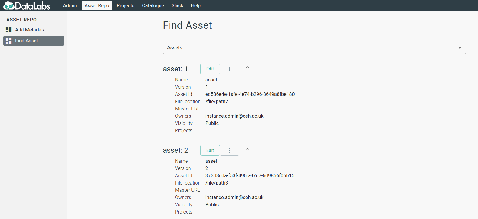
The following entries are associated with each entry;

• Name The name of the Asset.
• Version The version of the asset defined by the owner.
• Asset Id The internal ID of the dataset.
• File Location (For Admins) Where the data is stored on the storage server.
• Master URL Where you can find more about the data, or the original source of the data. This can be a DOI if the data is published elsewhere.
• Owners One or multiple users who are responsible for this asset within the DataLabs.
• Visibility Who can use this asset, either set to Public where anyone can access the data or By Project, where either one or a number of projects have access to the asset but no-one else.
• Projects If visibility is set to By Project, which projects can access the asset.

You can search the assets using the search box at the top, once you have selected an asset you are interested in, use the Master URL to find out more about it if relevant.

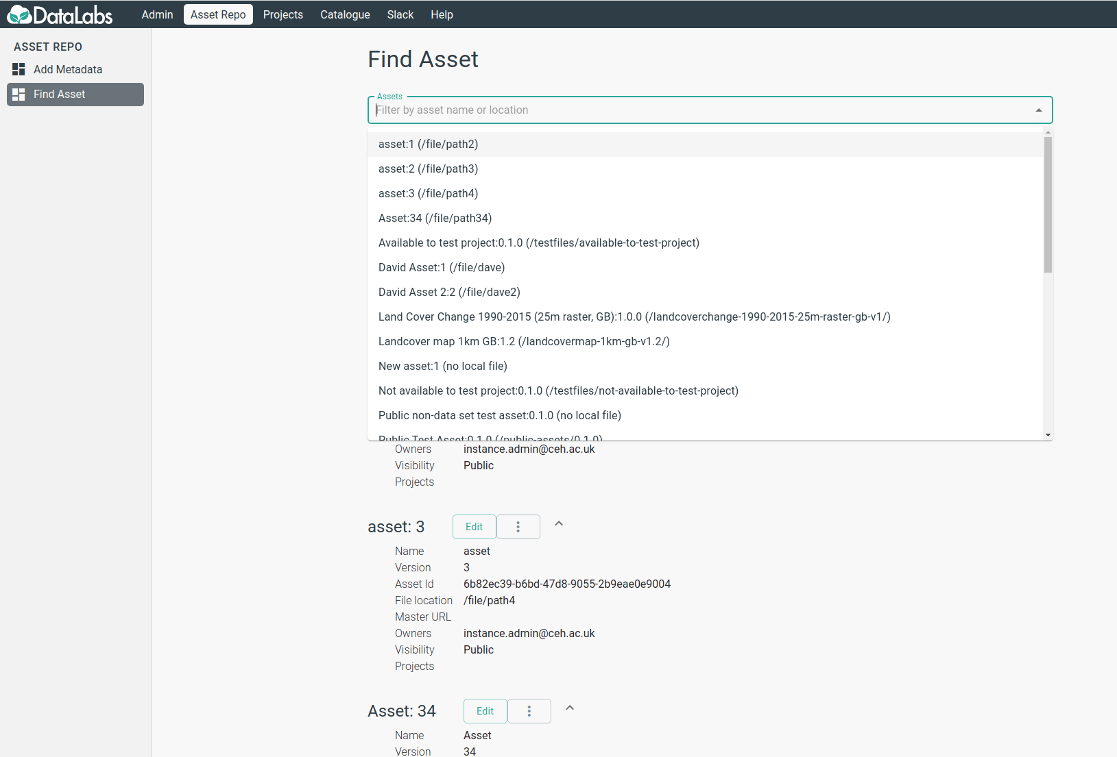
If you have found an asset you would like to utilize. You can use it by either;

• Selecting the ellipsis and Add to Notebook.
• Browsing to a notebook of yours and selecting the ellipsis followed by Edit, and adding the asset to the notebook. (NOTE: Doing this will restart the notebook so any unsaved work should be saved.)

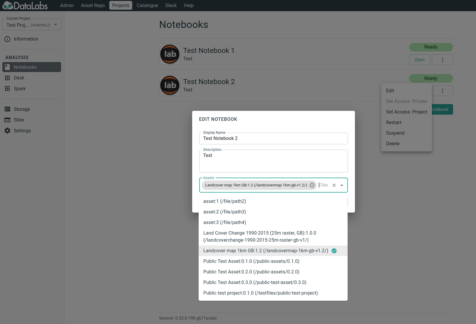
Once an asset is attached to a notebook, it will be accessible under within the assets folder at the base of the notebook. By default this will be done for all newly created notebooks.

Note when adding an asset to an older notebook prior to the release of the asset repo this can be replicated by creating a symbolic link yourself from the base of the notebook to the /assets folder as described below.

cd <Base Directory>
# For Jupyter this should be something like /data/notebooks/jupyterlab-<notebookname>
# or for RStudio the base of the project

ln -s /assets ./assets
# This creates a symbolic link from the base directory to the /assets mount point and
# allows it to be visible in the file pane

Can I request a new asset to be hosted?

Yes, if there is an asset you would like to use yourself or would be useful to the wider community get in touch with us on Slack or via e-mail. For certain datasets which are hosted e.g in the EIDC catalogue, there may be considerations around licensing which will prevent us from hosting a copy of the data however we will endeavor to help.

Can I submit my own assets to be hosted?

Yes, as with requesting a new asset we are able to accept your own data to be hosted in the Asset Repo and made available to others, get in touch with us directly to work this out.

Can I restrict assets data to my own project?

Yes, assets can be configured to be only accessible via specific projects if required.

Can I use assets within sites?

Yes, assets can be attached to sites and detached from sites.
Click to see the details

Attach/detach assets to/from site

In this tutorial, you will attach an asset during and after site creation and detach it from the site.

It is recommended that you should already be familiar with any one of the materials in the tutorial.
My first Panel site
or My first Voilà site
or My first Streamlit site

Attach an asset in creating site

From the "CREATE A SITE" popup, click on the "Assets" combo input to select an asset from the dropdown list or type in the combo input to select from a filtered list.

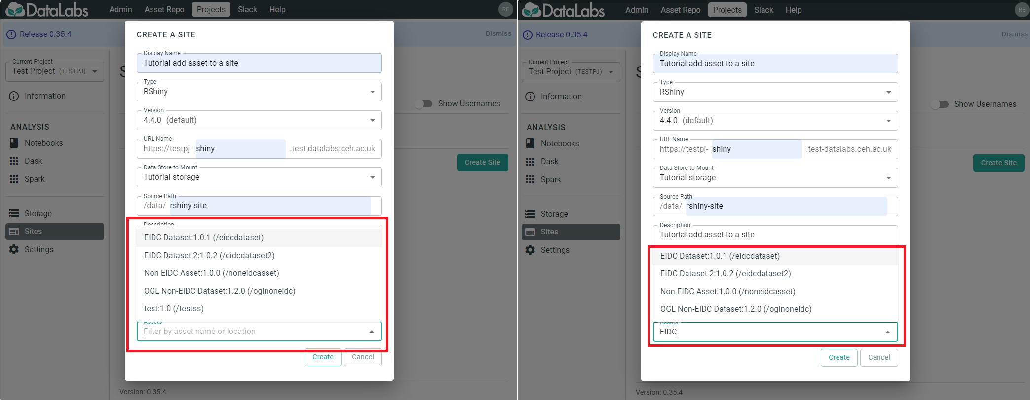
Attach an asset after site creation

From the "Sites" page, select the ellipsis and choose "Edit", in the "EDIT SITE" popup, click on the "Assets" combo input to select an asset from the dropdown list or type in the combo input to select from a filtered list. then click "Apply".

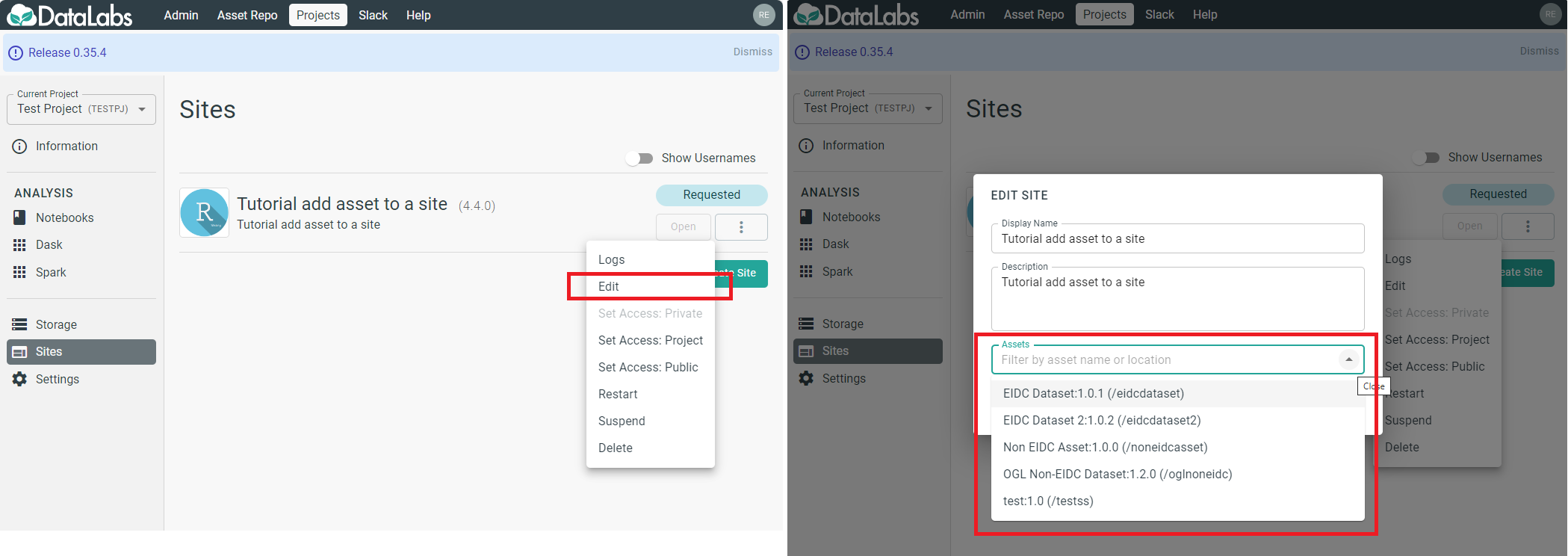
Detach an asset from a site

From the "Sites" page, select the ellipsis and choose "Edit", in the "EDIT SITE" popup, click on the cross icon by the asset to detach it from the site. then click "Apply".

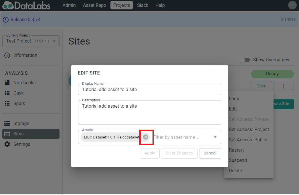
How to Suspend and Restart Resources

Why suspend my resources in DataLabs?

When not in active use, notebooks, sites and clusters use a minimal amount of resources. Suspending them frees up this resource to be used by others.

What does suspending a resource do?

Suspending a resource temporarily shuts it down. No existing data or configuration is lost. This takes a few minutes and will terminate the session of anyone using the resources. Once suspended, the resource can be turned back on when required.

Why are Notebooks automatically suspended?

Often people forget about resources they were previously working on. In order to prevent these resources draining capacity, a basic timeout policy is enforced which will automatically suspend notebooks. This comes into effect only if it has not been accessed (by a user opening the resource through DataLabs) for some time.

NOTE: This does not affect sites, which often sit idle for long periods of time for good reason.

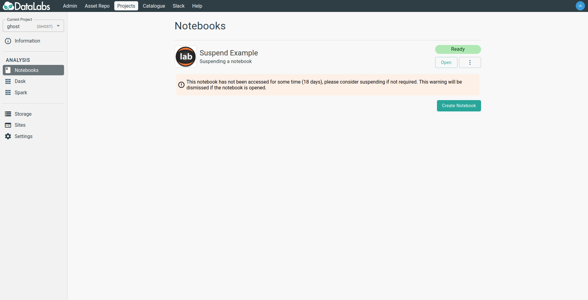
How will I know if a Notebook is about to be automatically suspended?

If a notebook has not been accessed in some time, a warning will be shown next to the notebook in question.

Can I manually suspend resources myself?

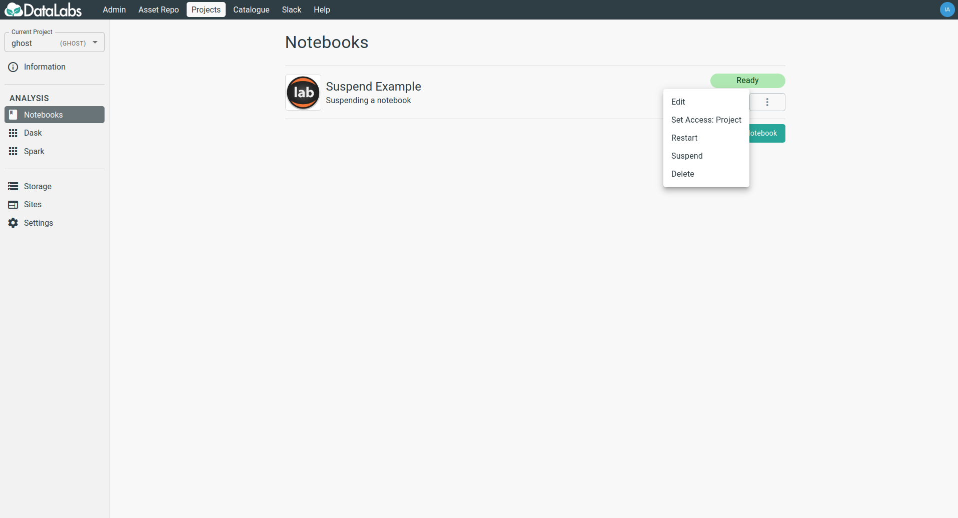
This is possible via the ellipsis button on the respective resources. The following can be manually suspended and restarted:

• Notebooks
• Sites
• Compute Clusters

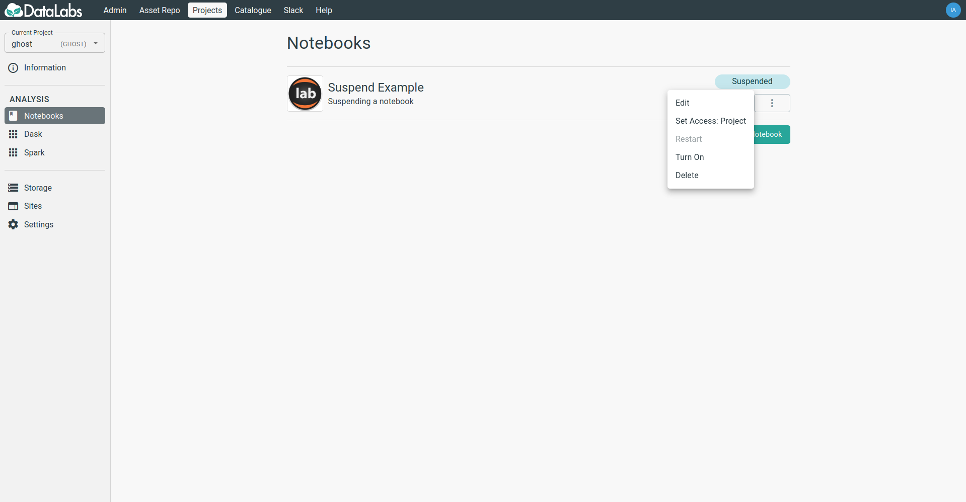
Once suspended, a resource can be restarted by any user with access to view it in a similar fashion.

I need a Notebook to remain running

Please get in touch with us via e-mail or Slack if you need your resource to continue running irrespective of access times.

Single user restriction of an RStudio notebook

An RStudio notebook can only be opened by one user at a time. This means that multiple users in a project cannot work on the same notebook simultaneously. The consequence of opening an RStudio notebook that someone else is currently using is to end their session.

How will I know if a notebook is in use

The link to an RStudio notebook will display a warning if it has been opened recently (eg within the last 8 hours). This indicates that it may be in use by another user. This is important because if you proceed to open the notebook then the current user will have their instance closed, causing some disruption to them.

What does this warning look like

Here is an example of what this warning looks like.

What should I do?

If you are aware of a colleague who may be using the notebook, it would be prudent to discuss the best way to work together on it.

Managing packages within R

In DataLabs, notebooks and services run as containers using linux based operating systems. When installing a R libary these packages are compiled and stored in a global library shared between the notebooks. As this library is shared packages may be updated, added or remove by other notebook users.

We recommend using packrat to manage the packages in a private library for each project and devtools to install specific versions, see Packrat Quick- Start Guide.

Package management on Spark with Packrat

Apache Spark is a distributed compute framework which runs numerous tasks in parallel across several worker nodes. Within DataLabs we have used Spark to solve large compute problems using the R language.

We have installed devtools and packrat on the worker nodes to enable management of packages on a project-by-project basis.

Using Packrat on the Spark cluster

Prerequisites

Firstly, initialise the project using Packrat (packrat::init) then install the required packages and finally update the lockfile with packrat::snapshot, see Packrat Quick-Start Guide.

Opening a project in a notebook with a Spark context

With using R in a Zeppelin notebook or a Jupyer notebook using R (SparkR) kernel the Spark context has been automatically generated and the SparkR loaded. To prevent Packrat from unloading this library the project must be opened using the clean.search.path = FALSE argument.

setwd('/data/example_project')
packrat::on(clean.search.path = FALSE)

Install R packages in a function running on spark

In DataLabs, the /data directory is shared between the Spark worker nodes and the notebooks. Running packrat::restore will compile and install any missing packages from the lockfile. These packages are stored within the private project library, therefore should only need to be build once as it is a shared directory.

sparkFunct <- function(idx) {
    # Open project
    setwd('/data/example-project')
    packrat::on(clean.search.path = FALSE)

    # Install if needed
    packrat::restore()

    # Run code on cluster
    library(fortunes)
    return(fortune())
}

spark.lapply(seq(4), sparkFunct)

In a multi-node cluster, it is possible the that many nodes will race to build the same package in an identical location, to prevent this run the spark function once (using a sequence of length 1) before running it with a larger sequence.

RStudio

In current releases of RStudio there is native integration between Packrat and RStudio projects which makes the management of dependecies with packrat easier.

New Projects

When creating a new project in RStudio, a checkbox can be selected which states Use packrat with this project, this will automatically initialise packrat in the RStudio session and create the folder structure for packrat by default.

Existing Projects

If you wish to convert to using Packrat with a current project in RStudio, this is possible by using the file browser in RStudio to select the directory which contains the project and navigating to;

Settings > Tools > Project Options > Packrat > 'Use packrat with this project'

This will automatically install the current packages in the project into a packrat directory and enable usage of the UI to manage packages via Packrat.

Managing packages within Conda

These pages describe how to use Conda environments within Jupyter for dependency management within DataLabs.

Adding & Removing Conda Packages

When using Conda within Jupyter, there a number of ways in which packages can be installed. When using Conda environments however it is important that packages are installed into the correct environment, hence there are a few recommended methods listed below.

Python

Python has native Conda Environment support. Hence from within a notebook using a specific Kernel simply calling conda install will automatically install the package into the current environment. This can also be desirable in a notebook to capture package installs for ease of reproducibility for others not working in the same environment.

Terminal

Conda packages can be installed from a Terminal session, however before carrying out the installs environmental variables must be setup to ensure packages are installed into the correct location, this process is a simple case of running source on the environment directory before proceeding with the installs.

source activate /data/conda/<environment_name>
conda install -y <package>

R

By default there is no native integration allowing Conda to be used from an R session, hence it is recommended that the terminal is used to install R packages. The majority of R packages should be available from the Conda repositories, however all are prefixed with r-, hence to install a package such as nycflights13, the following input will work.

source activate /data/conda/<environment_name>
conda install -y r-nycflights13

Using Object Storage within DataLabs

These pages describe how to interact with Object Storage from within Notebook sessions.

Increasingly object storage is being used to address an issue with the storage, this is for a number of reasons, a good review on the topic can be found here.

Within the DataLab environment, object storage is extremely useful as a place to store files that are;

• Of a big size (the architecture of object storage allows much easier scaling that traditional file storage).
• Unlikely to change. Object Storage is most performant primarily when reading files, hence this pattern works best when accessing the same files multiple times. This is often true for datasets which once produced/taken do not change.

For files that do not meet this criteria, particularly ones that require a lot of interaction with such as scripts or notebooks, it is recommended to carry on using the standard file storage provided within the labs which used by default and available at /data within the notebooks.

Getting Access

Before being able to access the object store, you must have valid user credentials. These will generally be associated with your JASMIN account and will be in the form of 2 strings, a secret key and an access key. Both of these should be kept securely.

Currently the only way to get credentials is to speak to the team, however this process is expected to be part of the standard JASMIN services portal soon.

Python

When accessing object storage with python there are a number of different libraries than can be used. This guide will focus on a standard library boto3. The general process is the same for other libraries.

Setup

The following describes one way to configure the boto3 library to use the credentials and endpoint as well as some basic activities such as downloading, uploading, listing.

# Set up the library and configuration
# The ACCESS_KEY, ACCESS_SECRET, and ENDPOINT will be provided when access
# is granted.
import boto3
session = boto3.session.Session()
s3_client = session.client(
  service_name='s3',
  aws_access_key_id=ACCESS_KEY,
  aws_secret_access_key=ACCESS_SECRET,
  endpoint_url=ENDPOINT
)

Buckets

Listing buckets

response = s3_client.list_buckets()
for bucket in response['Buckets']:
    print(bucket['Name'])

Making buckets

s3_client.create_bucket(Bucket='my-new-bucket')

List contents of bucket

response = s3_client.list_objects(Bucket=BUCKET_NAME)
print(response)

Files

Download File

# Key is the name of the file in the bucket you wish to download, and Filename
# is the name of the resulting file that will be saved in the local directory
s3_client.download_file(
  Bucket=BUCKET_NAME,
  Key='exampleFile1',
  Filename='downloaded_file'
)

Upload File

# Filename is the path to the file to upload, Key is the name of the resulting
# uploaded file in the bucket specified.
s3_client.upload_file(
  Filename='downloaded_file',
  Key='exampleFile1_uploaded',
  Bucket=BUCKET_NAME,
)

File Contents Into Memory

# Rather than downloading the file, this reads the file directly into a
# variable
response = s3_client.get_object(
  Bucket=BUCKET_NAME,
  Key='exampleFile1_uploaded'
)
var=response['Body']

Further Reading

Boto3 is a common library for which there is a lot of available documentation, this can be found here

Terminal

There are a number of different command line tools that can be used from within the labs to access/use the object storage, this will focus on using s3cmd.

Installation

s3cmd is a common OS package that should be available via standard repositories, hence from a Terminal session in Jupyter for example;

sudo apt update && sudo apt install -y s3cmd

Setup

Once installed, s3cmd can be configured interactively as follows;

$ s3cmd --configure

Enter new values or accept defaults in brackets with Enter.
Refer to user manual for detailed description of all options.

Access key and Secret key are your identifiers for Amazon S3. Leave them empty
for using the env variables.
Access Key []:
...

Ensure the correct values are entered when prompted - the main options which will be configured are Access Key, Secret Key, and S3 Endpoint.

Once this is complete, the output will be written to ~/.s3cfg

Usage

s3cmd usage is relatively simple and copies the usage of many standard POSIX commands and can be found with s3cmd --help, some simple examples are below.

List Buckets

$ s3cmd ls
2019-03-21 15:41  s3://bucket1
2019-09-03 15:07  s3://bucket2
2019-08-28 08:06  s3://another-bucket

List Files in a Bucket

$ s3cmd ls s3://bucket1
2019-03-21 15:42        46   s3://bucket1/file-in-bucket1

Upload a File to a Bucket

s3cmd put another-file s3://bucket1
upload: 'another-file' -> 's3://bucket1/another-file'  [1 of 1]
 0 of 0     0% in    2s     0.00 B/s  done

Download a File from a Bucket

s3cmd get s3://bucket1/another-file
download: 's3://bucket1/another-file' -> './another-file'  [1 of 1]
 0 of 0     0% in    3s     0.00 B/s  done

Desktop Clients

There are desktop clients that can be used to interact with Object Storage, one example of this is CyberDuck.

These have not however been tested as of yet.

Using Dask within JupyterLab

Dask is a widely used library for parallel computing in Python, information regarding it can be found here.

Within DataLabs, the JupyterLab extension dask-labextension is installed by default, and hence can be used to deploy and use a Dask Cluster. This will be able to take advantage of the compute resources shared within the environment to aid in solving issues that are parallel in nature.

Creating a Cluster

There are two options for creating a Dask cluster from within JupyterLab that are listed below.

NOTE: Since the resources used are shared among all users of the platform, when finished with the current activity Dask Workers should be should be shut down.

JupyterLab Dask Extension

The recommended way to create a cluster is to use the JupyterLab interface to create a new cluster. This is done simply by selecting the Dask icon in the left hand sidebar and selecting +NEW. This may take a few seconds to initialize and should result in a cluster appearing in the Clusters screen which is titled something like KubeCluster 1.

At this point the Dask scheduler will be setup but no workers will be present, these are added by selecting SCALE and choosing a worker count. Once the worker count is selected it may take up to a minute for all of the workers to register correctly, at this point (with a notebook open), selecting the <> icon will generate and insert python code to create a client to access the Dask cluster.

When finished with current work, the workers can be deleted by selecting SHUTDOWN.

Manual Setup (Advanced)

Instead of using the Dask JupyerLab extension which uses a number of standard defaults to create a Dask cluster, the same operation can be done manually. Configuaration for this is slightly more complex but allows for a greater degree of control, including choice of a default docker image that the Dask workers use as well as setting custom environmental variables.

The documentation for this can be found here. One thing to note within DataLabs is that when creating a custom worker-spec.yml as per the examples, an additional field must be added to ensure that workers are provisioned correctly within the cluster, this is namespace: ${PROJECT_KEY}-compute where PROJECT_KEY is the name of the current DataLabs project. An example of spinning up a Dask cluster manually can be found below.

from dask_kubernetes import KubeCluster

cluster = KubeCluster.from_yaml('worker-spec.yml')
cluster.scale_up(1)
cluster.adapt(minimum=1, maximum=3)

Where the worker-spec.yml is as follows.

kind: Pod
metadata:
  # This line must be added in order for workers to be created
  namespace: testproject-compute
spec:
  restartPolicy: Never
  containers:
  - image: daskdev/dask:latest
    imagePullPolicy: IfNotPresent
    args:
    - dask-worker
    - --nthreads
    - '2'
    - --no-bokeh
    - --memory-limit
    - 4GB
    - --death-timeout
    - '60'
    name: dask
    env:
      - name: EXTRA_PIP_PACKAGES
        value: xarray zarr
    resources:
      limits:
        cpu: "2"
        memory: 4G
      requests:
        cpu: "2"
        memory: 4G

Common Issues

Below is a number of common encountered issues and answers with using Dask within DataLabs.

Numbers of workers

The number of workers should be chosen carefully in accordance with the requirements of the analysis. As resources are all shared within the cluster it's imporant to not create more workers than are required, and to shut them down when the work is finished to free up the resources for others to use.

If you are finding that the number of workers does not reach the number you have tried to provision, it's likely that all of the resources in the cluster are currently being used, hence do not try to add any further workers without contacting an administrator.

Python Libraries

Dask workers are provisioned with a number of libraries by default, commonly however additional packages will be needed as part of the analysis. When using these non-default libraries, you will need to ensure that they are installed in all of the worker nodes prior to running the analysis.

This can be done with the following example below, where generally pip or conda will be used to install any required packages and dependencies. (Note that before running this a Dask cluster will have to be spun up and a client defined.)

conda_packages = "zarr numpy"
pip_packages = "xarray"

def install_packages():
    import os
    os.system("conda install %s -c conda-forge -y" % conda_packages)
    os.system("pip install %s" % pip_packages)

client.run(install)

It's recommended that this cell is kept within the notebook itself as it will need to be re-run when the Dask cluster is recreated.

Using Spark within DataLabs

This is documentaion on Spark usage in DataLabs.

These pages describe how to create Spark jobs from Jupyter Notebooks within DataLabs.

Basic Spark job

In DataLabs, users can create Spark clusters from the notebooks in their sessions and submit jobs to them.

Create Notebook

Create a Jupyter notebook within your defined project. When the notebook is created the Spark properties needed for the Spark cluster to be created is dynamically loaded into the notebook environment.

Set env variable

import os
os.environ['PYSPARK_PYTHON'] = '/usr/bin/python3'

Create Spark session

from pyspark.sql import SparkSession
spark = SparkSession.builder.appName('Test').getOrCreate()

Sample Spark code

rdd = spark.sparkContext.parallelize(range(10000000))
rdd.sum()

Stop the Spark session

spark.stop()

Spark job with local master

In DataLabs, users can create Spark clusters from the notebooks in their sessions and submit jobs to them.

Create Notebook

Create a Jupyter notebook within your defined project. When the notebook is created the Spark properties needed for the Spark cluster to be created is dynamically loaded into the notebook environment.

Set env variable

import os
os.environ['PYSPARK_PYTHON'] = '/usr/bin/python3'

Create Spark session

from pyspark.sql import SparkSession
spark = SparkSession.builder.master('local').appName('Test').getOrCreate()

Read data from project datastore

df = spark.read.csv('cities.csv', header=True)

Dispaly the dataframe created

df.show()

Stop the Spark session

spark.stop()

Spark job using Data in Object Store

In DataLabs, users can create Spark clusters from the notebooks in their sessions and submit jobs to them. This page describe how a user can submit a Spark job using data stored in the Object Storage.

Prerequisites

The user would need to have first obtained the Object store credentials from the JASMIN support team. These would be in the form of two strings - an access key and a secret key. These should be stored securely.

Create Notebook

Create a Jupyter notebook within your defined project. When the notebook is created the Spark properties needed for the Spark cluster to be created is dynamically loaded into the notebook environment.

Set Object Store Credentials in the environment

import os
os.environ['PYSPARK_PYTHON'] = '/usr/bin/python3'
os.environ['ACCESS_KEY'] = "xxxxxxx"
os.environ['SECRET_KEY'] = "xxxxxxxxx"

Create Spark session

from pyspark.sql import SparkSession
spark = SparkSession.builder.appName('Cropnet') \
    .config("fs.s3a.access.key", os.environ.get('ACCESS_KEY')) \
    .config("fs.s3a.secret.key", os.environ.get('SECRET_KEY')) \
    .config("fs.s3a.endpoint", "http://ceh-datalab-U.s3-ext.jc.rl.ac.uk") \
    .config("fs.s3a.path.style.access", True) \
    .config("fs.s3a.impl", "org.apache.hadoop.fs.s3a.S3AFileSystem") \
    .getOrCreate()

Read data from the Object store

df = spark.read.csv('s3a://cropnet-test/crops.csv', inferSchema=True,header=True)

Dispaly the dataframe created

df.show()

Stop the Spark session

spark.stop()

SparkR with Project Datastore

This is documentation on how users can create Spark clusters from within R sessions in Jupyter notebooks and submit jobs to them using the project datastore.

Create Notebook, Conda Environment and Select R Kernel

Create a Jupyter notebook within your defined project. When the notebook is created the Spark properties needed for the Spark cluster to be created is dynamically loaded into the notebook environment. Install a conda enviroment using https://datalab-docs.datalabs.ceh.ac.uk/conda-pkgs/conda_environments.html and select the R kernel.

Create Spark session

install.packages("SparkR")
library(SparkR, lib.loc = file.path(Sys.getenv('SPARK_HOME'), "R", "lib"))
sparkR.session(appname = "SparkR-Test",
               sparkHome = Sys.getenv("SPARK_HOME"),
               sparkConfig = list(spark.executor.instances = "6",
                                  spark.kubernetes.container.image = "nerc/sparkr-k8s:latest"))

Read data from project datastore

df <- read.df('cities.csv', header=True)

Dispaly the dataframe created

head(df)

Stop the Spark session

sparkR.session.stop()

SparkR with Object Store

This page describe how users can create Spark clusters from R sessions and submit jobs to them using data in the Object Store

Prerequisites

The user would need to have first obtained the Object store credentials from the JASMIN support team. These would be in the form of two strings - an access key and a secret key. These should be stored securely.

Create Notebook, Conda Environment and Select R Kernel

Create a Jupyter notebook within your defined project. When the notebook is created the Spark properties needed for the Spark cluster to be created is dynamically loaded into the notebook environment. Install a conda enviroment using https://datalab-docs.datalabs.ceh.ac.uk/conda-pkgs/conda_environments.html and select the Rkernel

Set Object Store Credentials in the environment

Sys.setenv(ACCESS_KEY = "xxxxxxx")
Sys.setenv(SECRET_KEY = "xxxxxxxxx")

Create Spark session

install.packages("SparkR")
library(SparkR, lib.loc = file.path(Sys.getenv('SPARK_HOME'), "R", "lib"))
sparkR.session(appName = "SparkR-Test",
               sparkHome = Sys.getenv("SPARK_HOME"),
               sparkConfig = list(spark.executor.instances = "2",
                                  spark.kubernetes.container.image = "nerc/sparkr-k8s:latest",
                                  fs.s3a.access.key = Sys.getenv("ACCESS_KEY"),
                                  fs.s3a.secret.key = Sys.getenv("SECRET_KEY"),
                                  fs.s3a.endpoint = "http://ceh-datalab-U.s3-ext.jc.rl.ac.uk",
                                  fs.s3a.path.style.access = "True",
                                  fs.s3a.impl = "org.apache.hadoop.fs.s3a.S3AFileSystem"))

Read data from the Object store

df <- read.df('s3a://spark-test/cities.csv', "csv", header = "true", inferSchema = "true",\
na.strings = "NA")

Dispaly the dataframe created

head(df)

Stop the Spark session

sparkR.session.stop()

Uploading files within DataLabs

When external data cannot be accessed externally it is often required for data to be brought into DataLabs.

For data that is available externally (for example by a direct download or API) it is recommended that data sets are downloaded directly into the lab environment using notebooks such as Jupyter/RStudio for purposes of ease.

This section will detail uploading data to the DataLabs storage either locally from a PC or some other source via Minio. (Note that for small files on the order of megabytes, these can be uploaded using Jupyter and RStudios respective 'upload' functions which work perfectly well).

Minio Client

The Minio client is a CLI tool that can be used to interact with Minio (upload and download files). This is a more robust solution in that it is able to upload larger files as well as having useful features such as resuming interrupted downloads.

In order to arrange to use this in DataLabs, first contact a DataLabs administrator who will enable this for your storage and provide credentials to access the storage remotely in the form of a secret key & an access key.

First download the Minio client. This is available for Linux, Windows & Mac. The below example shows a download of the Linux client.

wget https://dl.minio.io/client/mc/release/linux-amd64/mc
chmod +x mc

Once downloaded, use MC to add the host for the storage you wish to access & upload to. You will also need the URL of the Minio instance (can take this from the same URL used to access Minio and remove the trailing URL e.g https://project-storage.datalabs.ceh.ac.uk, make sure to replace the ACCESS_KEY and SECRET_KEY with those that were earlier provided.)

./mc --insecure config host add minio_storage \\
https://project-storage.datalabs.ceh.ac.uk $ACCESS_KEY $SECRET_KEY

Once mc is configured to point to the storage, it can be interacted with in a similar fashion to a standard UNIX file system. e.g

./mc --insecure ls minio_storage
./mc --insecure ls minio_storage/directory/
# Copy an example file in
./mc --insecure cp /tmp/local_file minio_storage/directory/
# Copy an entire directory in
./mc --insecure cp -r /tmp/localdirectory/ minio_storage/directory/

The full documentation for using mc can be found here - https://docs.min.io/docs/minio-client-complete-guide.html